At What Cost? Examining The Social Cost of Carbon

My testimony concerns the selective science that underlies the existing federal determination of the Social Cost of Carbon and how a more inclusive and considered process would have resulted in a lower value for the social cost of carbon.

Back in 2015, the federal government’s Interagency Working Group (IWG) on the Social Cost of Carbon released a report that was a response to public comments of the IWG’s determination of the social cost of carbon that were solicited by the Office of Management and Budget in November 2013. Of the 140 unique sets of substantive comments received (including a set of my own), the IWG adopted none. And apart from some minor updates to its discussion on uncertainty, the IWG, in its most recent August 2016 report, retained the same, now obsolete, methodologies that were used in its initial 2010 SCC determination.

Here, I address why this decision was based on a set of flimsy, internally inconsistent excuses and amounts to a continuation of the IWG’s exclusion of the most relevant science—an exclusion which assures that low, or even negative values of the social cost of carbon (which would imply a net benefit of increased atmospheric carbon dioxide levels), do not find their way into cost/benefit analyses of proposed federal actions. If, in fact, the social cost of carbon were near zero, it would eliminate the justification for any federal action (greenhouse gas emissions regulations, ethanol mandates, miles per gallon standards, solar/wind subsidies, DoE efficiency regulations, etc.) geared towards reducing carbon dioxide emissions.

Equilibrium Climate Sensitivity

In May 2013, the Interagency Working Group produced an updated SCC value by incorporating revisions to the underlying three Integrated Assessment Models (IAMs) used by the IWG in its initial 2010 SCC determination.  But, at that time, the IWG did not update the equilibrium climate sensitivity (ECS) employed in the IAMs. This was not done, despite, now, there having been, since January 1, 2011, at least 16 new studies and 32 experiments (involving more than 50 researchers) examining the ECS, each lowering the best estimate and tightening the error distribution about that estimate. Instead, the IWG wrote in its 2013 report: “It does not revisit other interagency modeling decisions (e.g., with regard to the discount rate, reference case socioeconomic and emission scenarios, or equilibrium climate sensitivity).”

This decision was reaffirmed by the IWG in July 2015 and again in its most recent August 2016 report. But, through its reaffirmation, the IWG has again refused to give credence to and recognize the importance of what is now becoming mainstream science—that the most likely value of the equilibrium climate sensitivity is lower than that used by the IWG and that the estimate is much better constrained. This situation has profound implications for the determination of the SCC and yet continues to be summarily dismissed by the IWG.

The earth’s equilibrium climate sensitivity is defined by the IWG in its 2010 report (hereafter, IWG2010) as “the long-term increase in the annual global-average surface temperature from a doubling of atmospheric CO2 concentration relative to pre-industrial levels (or stabilization at a concentration of approximately 550 parts per million (ppm))” and is recognized as “a key input parameter” for the integrated assessment models used to determine the social cost of carbon.

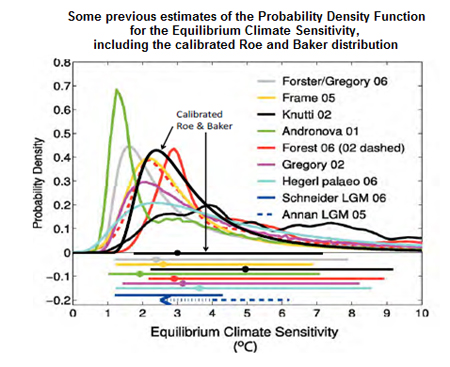
The IWG2010 report has an entire section (Section III.D) dedicated to describing how an estimate of the equilibrium climate sensitivity and the scientific uncertainties surrounding its actual value are developed and incorporated in the IWG’s analysis. The IWG2010, in fact, developed its own probability density function (pdf) for the ECS and used it in each of the three IAMs, superseding the ECS pdfs used by the original IAMs developers. The IWG’s intent was to develop an ECS pdf which most closely matched the description of the ECS as given in the Fourth Assessment Report of the United Nation’s Intergovernmental panel on Climate Change which was published in 2007.

The functional form adopted by the IWG2010 was a calibrated version of the Roe and Baker (2007) distribution.  It was described in the IWG2010 report in the following Table and Figure (from the IWG2010 report):

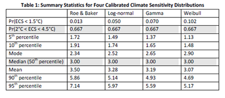
The calibrated Roe and Baker functional form used by the IWG2010 is no longer scientifically defensible; nor was it at the time of the publication of the IWG 2013 SCC update, nor at the time of the August 2016 update.

The figure below vividly illustrates this fact, as it compares the best estimate and 90% confidence range of the earth's ECS as used by the IWG (calibrated Roe and Baker) against findings in the scientific literature published since January 1, 2011.

Whereas the IWG ECS distribution has a median value of 3.0°C and 5th and 95th percentile values of 1.72°C and 7.14°C, respectively, the corresponding values averaged from the recent scientific literature are ~2.0°C (median), ~1.1°C (5th percentile), and ~3.5°C (95th percentile).

These differences will have large and significant impacts on the SCC determination.

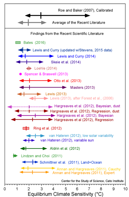
CAPTION: The median (indicated by the small vertical line) and 90% confidence range (indicated by the horizontal line with arrowheads) of the climate sensitivity estimate used by the Interagency Working Group on the Social Cost of Carbon Climate (Roe and Baker, 2007) is indicated by the top black arrowed line. The average of the similar values from 22 different determinations reported in the recent scientific literature is given by the grey arrowed line (second line from the top). The sensitivity estimates from the 32 individual determinations of the ECS as reported in new research published after January 1, 2011 are indicated by the colored arrowed lines. The arrows indicate the 5 to 95% confidence bounds for each estimate along with the best estimate (median of each probability density function; or the mean of multiple estimates; colored vertical line). Ring et al. (2012) present four estimates of the climate sensitivity and the red box encompasses those estimates. Likewise, Bates (2016) presents eight estimates and the green box encompasses them. Spencer and Braswell (2013) produce a single ECS value best-matched to ocean heat content observations and internal radiative forcing.

In addition to recent studies aimed at directly determining the equilibrium climate sensitivity (included in the chart above), there have been several other major studies which have produced results which qualitatively suggest a climate sensitivity lower than mainstream (e.g. Roe and Baker calibration) estimates. Such studies include new insights on cloud condensation nuclei and cosmic rays (Kirkby et al., 2016), radiative forcing of clouds (Bellouin, 2016; Stevens, 2015), cloud processes (Mauritsen and Stevens, 2015) and the underestimation of terrestrial CO2 uptake (Sun et al., 2014).

The IWG2010 report noted that, concerning the low end of the ECS distribution, its determination reflected a greater degree of certainty that a low ECS value could be excluded than did the IPCC. From the IWG2010 (p. 14):

“Finally, we note the IPCC judgment that the equilibrium climate sensitivity “is very likely larger than 1.5°C.” Although the calibrated Roe & Baker distribution, for which the probability of equilibrium climate sensitivity being greater than 1.5°C is almost 99 percent, is not inconsistent with the IPCC definition of “very likely” as “greater than 90 percent probability,” it reflects a greater degree of certainty about very low values of ECS than was expressed by the IPCC.”

In other words, the IWG used its judgment that the lower bound of the ECS distribution was higher than the IPCC 2007 assessment indicated. However, the collection of the recent literature on the ECS shows the IWG’s judgment to be in error. As can be seen in the chart above, the large majority of the findings on ECS in the recent literature indicate that the lower bound (i.e., 5th percentile) of the ECS distribution is lower than the IPCC 2007 assessment. And, the average value of the 5th percentile in the recent literature (~1.1°C) is 0.62°C less than that used by the IWG—a sizeable and important difference which will influence the SCC determination.

In fact, the abundance of literature supporting a lower climate sensitivity was at least partially reflected in the new IPCC assessment report issued in 2013. In that report, the IPCC reported:

Clearly, the IWG’s assessment of the low end of the probability density function that best describes the current level of scientific understanding of the climate sensitivity is incorrect and indefensible.

But even more influential in the SCC determination is the upper bound (i.e., 95th percentile) of the ECS probability distribution.

The IWG2010 notes (p.14) that the calibrated Roe and Baker distribution better reflects the IPCC judgment that “values substantially higher than 4.5°C still cannot be excluded.” The IWG2010 further notes that

In other words, the IWG2010 turned towards surveys of the scientific literature to determine its assessment of an appropriate value for the 95th percentile of the ECS distribution. Now, some seven years later, the scientific literature tells different story.

Instead of a 95th percentile value of 7.14°C, as used by the IWG2010, a survey of the recent scientific literature suggests a value of ~3.5°C—more than 50% lower.

And this is very significant and important difference because the high end of the ECS distribution has a large impact on the SCC determination—a fact frequently commented on by the IWG2010.

For example, from IWG2010 (p.26):

And further (p.30):

And the entirety of Section V “A Further Discussion of Catastrophic Impacts and Damage Functions” of the IWG 2010 report describes “tipping points” and “damage functions” that are probabilities assigned to different values of global temperature change. Table 6 from the IWG2010 indicated the probabilities of various tipping points.

The likelihood of occurrence of these low probability, high impact, events (“tipping points”) is greatly diminished under the new ECS findings. The average 95th percentile value of the new literature survey is only ~3.5°C indicating a very low probability of a warming reaching 3-5°C by 2100 as indicated in the 3rd column of the above Table and thus a significantly lower probability that such tipping points will be reached.  This new information will have a large impact on the final SCC determination using the IWG’s methodology.

The size of this impact has been directly investigated.

In their Comment on the Landmark Legal Foundation Petition for Reconsideration of Final Rule Standards for Standby Mode and Off Mode Microwave Ovens, Dayaratna and Kreutzer (2013) ran the DICE model using the distribution of the ECS as described by Otto et al. (2013)—a paper published in the recent scientific literature which includes 17 authors, 15 of which were lead authors of chapters in the recent Intergovernmental Panel on Climate Change’s Fifth Assessment Report. The most likely value of the ECS reported by Otto et al. (2013) was described as
“2.0°C, with a 5–95% confidence interval of 1.2–3.9°C.” Using the Otto et al. (2013) ECS distribution in lieu of the distribution employed by the IWG (2013), dropped the SCC by 42 percent, 41 percent, and 35 percent (for the 2.5%, 3.0%, 5.0% discount rates, accordingly). This is a significant decline.

In subsequent research, Dayaratna and Kreutzer (2014) examined the performance of the FUND (Framework for Uncertainty, Negotiation, and Distribution) model, and found that it too, produced a greatly diminished value for the SCC when run with the Otto et al. distribution of the equilibrium climate sensitivity. Using the Otto et al. (2013) ECS distribution in lieu of the distribution employed by the IWG (2013), dropped the SCC produced by the FUND model to $11, $6, $0 compared with the original $30, $17, $2 (for the 2.5%, 3.0%, 5.0% discount rates, accordingly). Again, this is a significant decline.

The Dayaratna and Kreutzer (2014) results using FUND were in line with alternative estimates of the impact of a lower climate sensitivity on the FUND model SCC determination.

Waldhoff et al. (2011) investigated the sensitivity of the FUND model to changes in the ECS.  Waldhoff et al. (2011) found that changing the ECS distribution such that the mean of the distribution was lowered from 3.0°C to 2.0°C had the effect of lowering the SCC by 60 percent (from a 2010 SCC estimate of $8/ton of CO2 to $3/ton in $1995). While Waldhoff et al. (2011) examined FUNDv3.5, the response of the current version (v3.8) of the FUND model should be similar.

Additionally, the developer of the PAGE (Policy Analysis of the Greenhouse Effect) model, affirmed that the SCC from the PAGE model, too drops by 35% when the Otto et al. (2013) climate sensitivity distribution is employed (Hope, 2013).

More recently, the FUND and DICE model were run with equilibrium climate sensitivities that were determined by Lewis and Curry (2014) in an analysis which updated and expanded upon the results of Otto et al. (2013). In Dayaratna et al. (2017), the probability density function (pdf) for the equilibrium climate sensitivity determined from an energy budget model (Lewis and Curry, 2014) was used instead of the Roe and Baker calibrated pdf used by the IWG. In doing so, Dayaranta et al. (2017) report:

These studies make clear that the strong dependence of the social cost of carbon on the distribution of the estimates of the equilibrium climate sensitivity (including the median, and the upper and lower certainty bounds) requires that the periodic updates to the IWG SCC determination must include a critical examination of the scientific literature on the topic of the equilibrium climate sensitivity, not merely kowtowing to the IPCC assessment. There is no indication that the IWG undertook such an independent examination. But what is clear, is that the IWG did not alter its probability distribution of the ECS between its 2010, 2013, 2015, and 2016 SCC determinations, despite a large and growing body of scientific literature that substantially alters and better defines the scientific understanding of the earth’s ECS. It is unacceptable that a supposed “updated” social cost of carbon does not include updates to the science underlying a critical and key aspect of the SCC.

I note that there has been one prominent scientific study in the recent literature which has argued, on the basis of recent observations of lower tropospheric mixing in the tropics, for a rather high climate sensitivity (Sherwood et al., 2014). This research, however, suffers from too narrow a focus. While noting that climate models which best match the apparent observed behavior of the vertical mixing characteristics of the tropical troposphere tend to be the models with high climate sensitivity estimates, the authors fail to make note that these same models are the ones whose projections make the worst match to observations of the evolution of global temperature during the past several decades.

While Sherwood et al. (2014) prefer models that better match their observations in one variable, the same models actually do worse in the big picture than do models which lack the apparent accuracy in the processes that Sherwood et al. (2014) describe. The result can only mean that there must still be even bigger problems with other model processes which must more than counteract the effects of the processes described by Sherwood et al.

This illustrates the inherent problems with “tuning” climate models to try to best reproduce a known set of observations—efforts to force climate models to better emulate one set of physical behaviors can degrade their performance on other ones. Voosen (2016) recently reported on the climate modelling community efforts to be more open and transparent with their multitude of (secret) “tuning” procedures. Voosen’s reporting was eye‐​opening not only in revealing the degree to which climate models are tuned and the significant role that tuning plays in model projections, but as to the reasons why modelers have not wanted to be up front about their methods. I reproduce an extended and relevant excerpt here:

That climate modelers were worried about being open about their methodologies for fear that “contrarians” would “unfairly” use such procedures against them indicates that the modeling community is more interested in climate policy (that may find support in their model projections) than climate science (which would welcome criticism aimed at producing a better understanding of the physical processes driving the earth’s climate). Given the degree of “secret sauce” mixed into the models at this point in time, a healthy dose of skepticsm regarding the verisimilitude of climate model output is warranted.

But even with the all the model tuning that takes place, the overall model collective is still warming the world much faster than it actually is. As shown by Christy (2016, and updates), there is a gross departure of “reality” from model predictions. Christy (2016) noted that “for the global bulk troposphere [roughly the bottom 40,000 feet of the atmosphere], the models overwarm the atmosphere by a factor of about 2.5.” The warming influence of a large and naturally occurring El Niño event has, temporarily, added a blip to the end of the observational record. But despite this short-term natural warming event, collectively the models still produce about twice as much warming as can be found in the real world over the past 38 years. And as the warming of the recent strong El Niño event fades (global surface temperatures have returned most of the way to pre-El Niño levels; see Figures below), the model/real world discrepancy will start to grow once again.

CAPTION: Five-year running mean temperatures predicted by the UN's climate models, and observed lower atmospheric temperatures from weather balloons and satellites (figure courtesy of John Christy).The last point is a four-year running mean, and the first two are three and four, respectively.

CAPTION: Monthly temperature anomalies, January 1997 through December 2016 (surface observations; top) and January 1997 through January 2017 (satellite observations of the mid-troposphere; bottom) show the impact of the strong 2016 El Niño event and the fading warmth since. The surface readings are from the Climate Research Unit at the University of East Anglia, and the satellite readings are from University of Alabama-Huntsville.

Another way to assess model performance is to compare model projection with observed trends in the vertical dimension of the atmosphere. Here again, as shown in the Figure below, models grossly produce much more warming than has been observed. This chart, courtesy of the University of Alabama at Huntsville’s Dr. John Christy, focuses on the tropics (between 20S and 20N)—the area where climate models project the greatest amount of warming through the atmosphere. The communal failure of the models is abject.

The characteristics of the vertical profile of temperature are important environmental variables  in that it is the vertical temperature distribution that determines atmospheric stability. When the lapse rate—the difference between the lowest layers and higher levels—is large, the atmosphere is unstable. Instability is the principal source for global precipitation. Although models can be (and are) tuned to mimic changes in surface temperatures, the same can’t be done as easily for the vertical profile of temperature changes. As the figure indicates, the air in the middle troposphere is warming far more slowly than has been predicted, even more slowly than the torpid surface warming.  Consequently, the difference between the surface and the middle troposphere has become slightly greater, a condition which should produce a very slight increase in average precipitation. On the other hand, the models forecast that the difference between the surface and the middle troposphere should become less, a condition which would add pressure to decrease global precipitation.

The models are therefore making systematic errors in their precipitation projections. That has a dramatic effect on the resultant climate change projections. When the surface is wet, which is what occurs after rain, the sun’s energy is directed toward the evaporation of that moisture rather than to directly heating the surface. In other words, much of what is called “sensible weather” (the kind of weather a person can sense) is determined by the vertical distribution of temperature. If the popular climate models get that wrong (which is what is happening), then all the subsidiary weather may also be incorrectly specified.

CAPTION: Tropical (20°S to 20°N) temperature trends(1979-2016) throughout the vertical atmosphere as projected by climate models (red squares, with uncertainty) and as observed by radiosondes carried aloft by weather balloons (colored circles represent different data compilations). The red line is the model mean and the green line is the observed mean. The trend in the bulk lower atmosphere (middle troposphere) from several different satellite data compilations (colored plus signs, top box) and several reanalysis datasets (colored crosses, top box) is compared with the model projection for the same layer in the box at the top of the figure. (Figure courtesy of John Christy)

These results argue strongly against the reliability of the Sherwood et al. (2014) conclusion and instead provide robust observational evidence that the climate sensitivity has been overestimated by both climate models, and the IWG alike.
Agricultural Impacts of Carbon Fertilization

Carbon dioxide is known to have a large positive impact on vegetation (e.g., Zhu et al., 2016), with literally thousands of studies in the scientific literature demonstrating that plants (including crops) grow stronger, healthier, and more productive under conditions of increased carbon dioxide concentration. A study (Idso, 2013) reviewed a large collection of such literature as it applies to the world's 45 most important food crops (making up 95% of the world's annual agricultural production).

Idso (2013) summarized his findings on the increase in biomass of each crop that results from a 300ppm increase in the concentration of carbon dioxide under which the plants were grown. This table is reproduced below, and shows that the typical growth increase exceeds 30% in most crops, including 8 of the world's top 10 food crops (the increase was 24% and 14% in the other two).

Idso (2013) found that the increase in the atmospheric concentration of carbon dioxide that took place during the period 1961-2011 was responsible for increasing global agricultural output by 3.2 trillion dollars (in 2004-2006 constant dollars). Projecting the increases forward based on projections of the increase in atmospheric carbon dioxide concentration, Idso (2013) expects carbon dioxide fertilization to increase the value of agricultural output by 9.8 trillion dollars (in 2004-2006 constant dollars) during the 2012-2050 period.

Average percentage increase in biomass of each of the world's 45 most important food crops under an increase of 300ppm of carbon dioxide.

This is a large positive externality, and one that is insufficiently modeled in the IAMs relied upon by the IWG in determining the SCC.

In fact, only one of the three IAMs used by the IWG has any substantial impact from carbon dioxide fertilization, and the one that does, underestimates the effect by approximately 2-3 times.

The FUND model has a component which calculates the impact on agricultural as a result of carbon dioxide emissions, which includes not only the impact on temperature and other climate changes, but also the direct impact of carbon dioxide fertilization. The other two IAMs, DICE and PAGE by and large do not (or only do so extremely minimally; DICE includes the effect to a larger degree than PAGE). Consequently, lacking this large and positive externality, the SCC calculated by the DICE and PAGE models is significantly larger than the SCC determined by the FUND model (for example, see Table A5, in the IWG 2013 report).

But even the positive externality that results from carbon dioxide fertilization as included in the FUND model is too small when compared with the Idso (2013) estimates. FUND (v3.7) uses the following formula to determine the degree of crop production increase resulting from atmospheric carbon dioxide increases (taken from Anthoff and Tol, 2013a):

Column 8 in the table below shows the CO2 fertilization parameter (γr) used in FUND for various regions of the world (Anthoff and Tol, 2013b). The average CO2 fertilization effect across the 16 regions of the world is 11.2%. While this number is neither areally weighted, nor weighted by the specific crops grown, it is clear that 11.2% is much lower than the average fertilization effect compiled by Idso (2013) for the world's top 10 food crops (35%). Further, Idso's fertilization impact is in response to a 300ppm CO2 increase, while the fertilization parameter in the FUND model is multiplied by ln(CO2t/275) which works out to 0.74 for a 300ppm CO2 increase. This multiplier further reduces the 16 region average to 8.4% for the CO2 fertilization effect—some 4 times smaller than the magnitude of the fertilization impact identified by Idso (2013).

Although approximately four times too small, the impact of the fertilization effect on the SCC calculation in the FUND model is large.

According to Waldhoff et al. (2011), if the CO2 fertilization effect is turned off in the FUND model (v3.5) the SCC increases by 75% from $8/tonCO2 to $14/tonCO2 (in 1995 dollars). In another study, Ackerman and Munitz (2012) find the effective increase in the FUND model to be even larger, with CO2 fertilization producing a positive externality of nearly $15/tonCO2 (in 2007 dollars).

Clearly, had the Idso (2013) estimate of the CO2 fertilization impact been used instead of the one used in FUND the resulting positive externality would have been much larger, and the resulting net SCC been much lower.

This is just for one of the three IAMs used by the IWG. Had the more comprehensive CO2 fertilization impacts identified by Idso (2013) been incorporated in all the IAMs, the three-model average SCC used by the IWG would be been greatly lowered, and likely even become negative in some IAM/discount rate combinations.

In its 2015 “Response to Comments Social Cost of Carbon for Regulatory Impact Analysis Under Executive Order 12866,” the IWG admits to the disparate ways that CO2 fertilization is included in the three IAMs. Nevertheless, the IWG quickly dismisses this as a problem in that they claim the IAMs were selected “to reflect a reasonable range of modeling choices and approaches that collectively reflect the current literature on the estimation of damages from CO2 emissions.”

This logic is blatantly flawed. Two of the IAMs do not reflect the “current literature” on a key aspect relating to the direct impact of CO2 emissions on agricultural output, and the third only partially so.

CO2 fertilization is a known physical effect from increased carbon dioxide concentrations.  By including the results of IAMs that do not include known processes that have a significant impact on the end product must disqualify them from contributing to the final result. The inclusion of results that are known a priori to be wrong can only contribute to producing a less accurate answer. Results should only be included when they attempt to represent known processes, not when they leave those processes out entirely.

The justification from the IWG (2015) that “[h]owever, with high confidence the IPCC (2013) stated in its Fifth Assessment Report (AR5) that ‘[b]ased on many studies covering a wide range of regions and crops, negative impacts of climate change on crop yields have been more common than positive ones’” is completely irrelevant as CO2 fertilization is an impact that is apart from “climate change.” And further, the IAMs do (explicitly in the case of FUND and DICE or implicitly in the case of PAGE) include damage functions related to the climate change impacts on agriculture. So not only is the IWG justification irrelevant, it is inaccurate as well. The impact of CO2 fertilization on agricultural output and its impact on lowering the SCC must be considered.

Additional Climate Model Parameter Misspecifications

In addition to the outdated climate sensitivity distribution and the insufficient handling of the carbon dioxide fertilization effect, there has also been identified a misspecification of some of the critical parameters within the underlying box models that drive the pace and shape of the future climate evolution in the IAMs.

A recent analysis (Lewis, 2016) finds that the physically-based two-box climate model inherent in the DICE IAM is fit with physically unrealistic ocean characteristics. According to Lewis (2016):

When the DICE 2‑box model is parametrized with values for the ocean layers that are in line with established estimates, the value of the social cost of carbon that results is reduced by one‐​quarter to one‐​third during the 21th century. Lewis further point out that notes that “The climate response profile in FUND and in PAGE, the other two IAMs used by the US government to assess the SCC, appear to be similarly inappropriate, suggesting that they also overestimate the SCC.”

Ultimately, Lewis (2016) concludes:

Sea Level Rise

The sea level rise module in the DICE model used by the IWG2013/2015/2016 produces future sea level rise values that far exceed mainstream projections and are unsupported by the best available science. The sea level rise projections from more than half of the scenarios (IMAGE, MERGE, MiniCAM) exceed even the highest end of the projected sea level rise by the year 2300 as reported in the Fifth Assessment Report (AR5) of the Intergovernmental Panel on Climate Change (see figure).

CAPTION: Projections of sea level rise from the DICE model (the arithmetic average of the 10,000 Monte Carlo runs from each scenario ) for the five scenarios examined by the IWG2013 compared with the range of sea level rise projections for the year 2300 given in the IPCC AR5 (see AR5 Table 13.8). (DICE data provided by Kevin Dayaratna and David Kreutzer of the Heritage Foundation).

How the sea level rise module in DICE was constructed is inaccurately characterized by the IWG (and misleads the reader).  The IWG report describes the development of the DICE sea level rise scenario as:

However, in IWG footnote “6” the methodology is described this way (Nordhaus, 2010):

“Using estimates” and “calibrating” are two completely different things. Calibration implies that the sea level rise estimates produced by the DICE sea level module behave similarly to the IPCC sea level rise projections and instills a sense of confidence in the casual reader that the DICE projections are in accordance with IPCC projections. However this is not the case. Consequently, the reader is misled.

In fact, the DICE estimates are much higher than the IPCC estimates. This is even recognized by the DICE developers. From the same reference as above:

That the DICE sea level rise projections are far above mainstream estimated can be further evidenced by comparing them with the results produced by the IWG-accepted MAGICC modelling tool (in part developed by the EPA and available from http://www.cgd.ucar.edu/cas/wigley/magicc/).

Using the MESSAGE scenario as an example, the sea level rise estimate produced by MAGICC for the year 2300 is 1.28 meters—a value that is less than 40% of the  average value of 3.32 meters produced by the DICE model when running the same scenario (see figure below).

CAPTION: Projected sea level rise resulting from the MESSAGE scenario produced by DICE (red) and MAGICC (blue).

The justification given for the high sea level rise projections in the DICE model (Nordhaus, 2010) is that they well-match the results of a “semi-empirical” methodology employed by Rahmstorf (2007) and Vermeer and Rahmstorf (2009).

However, subsequent science has proven the “semi-empirical” approach to projecting future sea level rise unreliable. For example, Gregory et al. (2012) examined the assumption used in the “semi-empirical” methods and found them to be unsubstantiated. Gregory et al (2012) specifically refer to the results of Rahmstorf (2007) and Vermeer and Rahmstorf (2009):

In light of these findings, the justification for the very high sea level rise projections (generally exceeding those of the IPCC AR5 and far greater than the IWG‐​accepted MAGICC results) produced by the DICE model is called into question and can no longer be substantiated.

Given the strong relationship between sea level rise and future damage built into the DICE model, there can be no doubt that the SCC estimates from the DICE model are higher than the best science would allow and consequently, should not be accepted by the IWG as a reliable estimate of the social cost of carbon.

And here again, the IWG (2015) admits that these sea level rise estimates are an outlier on the high end, yet retains them in their analysis by claiming than they were interested in representing a “range” of possible outcomes. But, even the IWG (2015) admits that the IPCC AR5 assigned “a low confidence in projections based on such [semi‐​empirical] methods.” It is internally inconsistent to claim the IPCC as an authority for limiting the range of possibilities explored by the IAMs (which it did in the case of equilibrium climate sensitivity) and then go outside the IPCC to justify including a wildly high estimate of sea level rise. Such inconsistencies characterize the IWG response to comments and weaken confidence in them.

I did not investigate the sea level rise projections from the FUND or the PAGE model, but suggest that such an analysis must be carried out prior to extending any confidence in the values of the SCC resulting from those models—confidence that, as demonstrated, cannot be assigned to the DICE SCC determinations.

Conclusion

The social cost of carbon as determined by the Interagency Working Group in their August 2016 Technical Support Document (updated from IGW reports from February 2010, November 2013, and July 2015) is unsupported by the robust scientific literature, fraught with uncertainty, illogical, and thus completely unsuitable and inappropriate for federal rulemaking. Had the IWG included a better‐​reasoned and more inclusive review of the current scientific literature, the social cost of carbon estimates would have been considerably reduced with a value likely approaching zero. Such a low social cost of carbon would obviate the arguments behind the push for federal greenhouse gas regulations.

References

Ackerman, F., and C. Munitz, 2012. Climate damages in the FUND model: a disaggregated analysis. Ecological Economics, 77, 219–224.

Aldrin, M., et al., 2012. Bayesian estimation of climate sensitivity based on a simple climate model fitted to observations of hemispheric temperature and global ocean heat content. Environmetrics, doi: 10.1002/env.2140.

Annan, J.D., and J.C Hargreaves, 2011. On the genera­tion and interpretation of probabilistic estimates of climate sensitivity. Climatic Change, 104, 324–436.

Anthoff, D., and R.S.J. Tol, 2013a. The climate framework for uncertainty, negotiation and distribution (FUND), technical description, version 3.7, http://​www​.fund​-mod​el​.org/​p​u​b​l​i​c​a​tions

Anthoff, D., and R.S.J. Tol, 2013b. The climate framework for uncertainty, negotiation and distribution (FUND), tables, version 3.7, http://​www​.fund​-mod​el​.org/​p​u​b​l​i​c​a​tions

Bates, J. R., 2016. Estimating Climate Sensitivity Using Two‐​zone Energy Balance Models. Earth and Space Science, doi: 10.1002/2015EA000154

Bellouin, N., 2016. The interaction between aerosols and clouds. Weather and Climate @Reading, http://​blogs​.read​ing​.ac​.uk/​w​e​a​t​h​e​r​-​a​n​d​-​c​l​i​m​a​t​e​-​a​t​-​r​e​a​d​i​n​g​/​2​0​1​6​/​1053/.

Christy, J.R., 2016. Testimony before the House Committee on Science, Space, and Technology, February 2, 2016.

Dayaratna, K., and D. Kreutzer, 2013. Comment on the Energy Efficiency and Renewable Energy Office (EERE) Proposed Rule: 2013-08-16 Energy Conservation Program for Consumer Products: Landmark Legal Foundation; Petition for Reconsideration; Petition for Reconsideration; Request for Comments, http://www.regulations.gov/#!documentDetail;D=EERE-2013-BT-PET-0043–0024

Dayaratna, K., and D. Kreutzer, 2014. Unfounded FUND: Yet another EPA model not ready for the Big Game, http://​www​.her​itage​.org/​r​e​s​e​a​r​c​h​/​r​e​p​o​r​t​s​/​2​0​1​4​/​0​4​/​u​n​f​o​u​n​d​e​d​-​f​u​n​d​-​y​e​t​-​a​n​o​t​h​e​r​-​e​p​a​-​m​o​d​e​l​-​n​o​t​-​r​e​a​d​y​-​f​o​r​-​t​h​e​-​b​i​g​-game.

Dayaratna, K., R. McKitrick, and D. Kreutzer, 2017. Empirically‐​constrained climate sensitivity and the social cost of carbon. Accepted, Climate Change Economics.

Gregory, J., et al., 2012. Twentieth‐​century global‐​mean sea‐​level rise: is the whole greater than the sum of the parts? Journal of Climate, doi:10.1175/JCLI-D-12–00319.1, in press.

Hargreaves, J.C., et al., 2012. Can the Last Glacial Maximum constrain climate sensitivity? Geophysical Research Letters, 39, L24702, doi: 10.1029/2012GL053872

Hope, C., 2013. How do the new estimates of transient climate response affect the social cost of CO2? http://​www​.chrish​ope​pol​i​cy​.com/​2​0​1​3​/​0​5​/​h​o​w​-​d​o​-​t​h​e​-​n​e​w​-​e​s​t​i​m​a​t​e​s​-​o​f​-​t​r​a​n​s​i​e​n​t​-​c​l​i​m​a​t​e​-​r​e​s​p​o​n​s​e​-​a​f​f​e​c​t​-​t​h​e​-​s​o​c​i​a​l​-​c​o​s​t​-​o​f​-co2/ (last visited May 5, 2014)

Idso, C. 2013. The positive externalities of carbon dioxide: Estimating the monetary benefits of rising CO2 concentrations on global food production. Center for the Study of Carbon Dioxide and Global Change, 30pp.

Intergovernmental Panel on Climate Change, 2007. Climate Change 2007: The Physical Science Basis. Contribution of Working Group I to the Fourth Assessment Report of the Intergovernmental Panel on Climate Change. Solomon, S., et al. (eds). Cambridge University Press, Cambridge, 996pp.

Intergovernmental Panel on Climate Change, 2013. Climate Change 20013: The Physical Science Basis. Contribution of Working Group I to the Fifth Assessment Report of the Intergovernmental Panel on Climate Change. Final Draft Accepted in the 12th Session of Working Group I and the 36th Session of the IPCC on 26 September 2013 in Stockholm, Sweden.

Kirkby, J., et al., 2016. Ion‐​induced nucleation of pure biogenic particles. Nature, 533, 521–526, doi:10.1038/nature17953.

Lewis, N. 2013. An objective Bayesian, improved approach for applying optimal fingerprint techniques to estimate climate sensitivity. Journal of Climate, doi: 10.1175/JCLI-D-12–00473.1.

Lewis, N. and J.A. Curry, C., 2014. The implications for climate sensitivity of AR5 forcing and heat uptake estimates. Climate Dynamic, 10.1007/s00382-014‑2342‑y.

Lewis, N., 2016. Abnormal climate response of the DICE IAM – a trillion dollar error? Climate Etc., last accessed, August 16, 2016, https://​judithcur​ry​.com/​2​0​1​6​/​0​8​/​1​5​/​a​b​n​o​r​m​a​l​-​c​l​i​m​a​t​e​-​r​e​s​p​o​n​s​e​-​o​f​-​t​h​e​-​d​i​c​e​-​i​a​m​-​a​-​t​r​i​l​l​i​o​n​-​d​o​l​l​a​r​-​e​rror/

Lindzen, R.S., and Y‑S. Choi, 2011. On the observational determination of climate sensitivity and its implica­tions. Asia‐​Pacific Journal of Atmospheric Science, 47, 377–390.

Loehle, C., 2014. A minimal model for estimating climate sensitivity. Ecological Modelling, 276, 80–84.

Masters, T., 2013. Observational estimates of climate sensitivity from changes in the rate of ocean heat uptake and comparison to CMIP5 models. Climate Dynamics, doi:101007/s00382-013‑1770‑4

Mauritsen, T. and B. Stevens, 2015. Missing iris effect as a possible cause of muted hydrological change and high climate sensitivity in models. Nature Geoscience, 8, 346–351, doi:10.1038/ngeo2414.

Nordhaus, W., 2010. Projections of Sea Level Rise (SLR), http://www.econ.yale.edu/~nordhaus/homepage/documents/SLR_021910.pdf

Otto, A., F. E. L. Otto, O. Boucher, J. Church, G. Hegerl, P. M. Forster, N. P. Gillett, J. Gregory, G. C. Johnson, R. Knutti, N. Lewis, U. Lohmann, J. Marotzke, G. Myhre, D. Shindell, B. Stevens, and M. R. Allen, 2013. Energy budget constraints on climate response. Nature Geoscience, 6, 415–416.

Rahmstorf, S., 2007. A semi‐​empirical approach to projecting future sea‐​level rise. Science, 315, 368–370, doi:10.1126/science.1135456.

Ring, M.J., et al., 2012. Causes of the global warming observed since the 19th century. Atmospheric and Climate Sciences, 2, 401–415, doi: 10.4236/acs.2012.24035.

Schmittner, A., et al. 2011. Climate sensitivity estimat­ed from temperature reconstructions of the Last Glacial Maximum. Science, 334, 1385–1388, doi: 10.1126/science.1203513.

Sherwood, S. C., S. Bony, and J‑D. Dufresne, 2014. Spread in model climate sensitivity traced to atmospheric convective mixing. Nature, 505,37–42, doi:10.1038/nature12829.

Skeie, R. B., T. Berntsen, M. Aldrin, M. Holden, and G. Myhre, 2014. A lower and more constrained estimate of climate sensitivity using updated observations and detailed radiative forcing time series. Earth System Dynamics, 5, 139–175.

Spencer, R. W., and W. D. Braswell, 2013. The role of ENSO in global ocean temperature changes during 1955–2011 simulated with a 1D climate model. Asia‐​Pacific Journal of Atmospheric Science, doi:10.1007/s13143-014‑0011‑z.

Stevens, B., 2015. Rethinking the lower bound on aerosol radiative forcing. Journal of Climate, 28, 4794–4819, doi: 10.1175/JCLI-D-14–00656.1.

Sun, Y., et al., 2014. Impact of mesophyll diffusion on estimated global land CO2 fertilization. Proceedings of the National Academy of Science, 111, 15774–15779, doi: 10.1073/pnas.1418075111.

van den Bergh, J.C.J.M., and W.J.W. Botzen, 2014. A lower bound to the social cost of CO2 emissions. Nature Climate Change, 4, 253–258, doi:10.1038/NCLIMATE2135.

Vermeer, M. and S. Rahmstorf, 2009. Global sea level linked to global temperature. Proceedings of the National Academy of Sciences, 106, 51, 21527–21532, doi:10.1073/pnas.0907765106.

Voosen, P., 2016. Climate scientists open up their black boxes to scrutiny. Science, 354, 401–402.

Waldhoff, S., Anthoff, D., Rose, S., and R.S.J. Tol, 2011. The marginal damage costs of different greenhouse gases: An application of FUND. Economics, The Open‐​Access E‑Journal, No. 2011–43, http://www.economics-ejournal.org/economics/discussionpapers/2011–43

Wigley, T.M.L., et al. MAGICC/SCENGEN v5.3. Model for the Assessment of Greenhouse‐​gas Induced Climate Change/​A Regional Climate Scenario Generator. http://​www​.cgd​.ucar​.edu/​c​a​s​/​w​i​g​l​e​y​/​m​a​gicc/

Zhu, Z., et al., 2016. Greening of the Earth and its drivers. Nature Climate Change, doi: 10.1038/nclimate3004