With revenue growth flagging, now is a good time for states to look for budgetary savings. In this study, I find limited evidence that greater program spending correlates with better social outcomes, so state governments should be able to make extensive spending cuts without jeopardizing the quality of core services.

Opportunities for cost savings can be found in higher education, and, to a lesser extent, in K–12 education, where merging underutilized colleges and schools can lower administrative costs while freeing up valuable real estate.

States should also avoid overinvestments in public transit, which has seen decreased ridership in the aftermath of COVID-19. A survey of recent transit infrastructure projects shows that many are affected by large cost overruns and significant implementation delays. When combined with lower‐​than‐​expected ridership, these projects usually do not provide sufficient benefits to justify their enormous costs.

Relative to the federal government, most states enjoy low debt burdens. To keep it that way, states should avoid issuing new bonds, especially during this time of high interest rates. They should also trim retiree health benefits and adopt more conservative return assumptions for pension plan assets.

This study considers other state spending programs and offers additional suggestions for prudently reducing spending.

Most state governments have emerged from the COVID-19 pandemic in a stronger financial position than they entered it. They benefited from unexpectedly high tax receipts, low borrowing rates, and hundreds of billions of federal rescue funds. As the Federal Reserve raises debt servicing costs and crimps economic growth, and as we enter a period of divided federal governance, these tailwinds are ending or even reversing. Going forward, states will have to control spending and the growth of liabilities to maintain fiscal stability. High‐​tax states will also be more vulnerable to competition for taxpayers from lower‐​tax jurisdictions as the number of retirees increases and remote work becomes normalized.

This analysis begins with an overview of state fiscal conditions in the pandemic’s aftermath, and then moves on to a discussion of the main categories of state spending as identified by the National Association of State Budget Officers (NASBO). It concludes with a series of incremental policy recommendations to state governments that are interested in preserving fiscal sustainability and improving their competitiveness. An appendix investigates the relationship between four categories of state spending (Medicaid, K–12 Education, Higher Education, and Transportation) and policy outcomes. These analyses do not suggest strong correlations between spending and outcomes.

By early 2022, state tax revenues had fully recovered from the pandemic recession. Only two states, North Dakota and Wyoming, reported tax revenues below 2019 levels on an inflation‐​adjusted basis. States exhibiting especially strong revenue growth were those that experienced high in‐​migration, such as Idaho and Utah, and those that have progressive income tax rates and numerous high‐​income earners, such as New York and California.¹

Monthly cash reports from state fiscal year 2023 show weakening revenue performance in New York and California.² This finding tracks with more pessimistic budget forecasts from the California Legislative Analyst’s Office and the New York State Comptroller.³ States dependent on income tax revenue from high earners are prone to wide swings in collections coinciding with stock market movements, since many high earners receive equity‐​based compensation and/​or earn substantial income from capital gains.

Strong revenues allowed states to replenish rainy day funds that were drawn down at the beginning of the pandemic. Median state rainy day fund balances reached a record 42.5 days of state expenditures at the end of fiscal year 2022, according to Pew Charitable Trust data. That is double fiscal year (FY) 2017 levels.⁴ Considering all forms of cash reserves, the picture is even brighter, with the median state reporting resources equal to 88.9 days of spending at the end of FY 2022, although this is slightly down from FY 2021.

In March 2021, President Biden signed the American Rescue Plan Act (ARPA), which included $195.3 billion of recovery funds for states and an additional $4.5 billion for the District of Columbia and US territories.

According to a National Association of State Budget Officers evaluation of state ARPA disclosures, states had budgeted 80 percent of the funds they had received under this program, leaving less than $40 billion unallocated.⁵ The state budgetary tailwind provided by ARPA is thus largely exhausted. If a recession develops in 2024 states will face renewed fiscal pressure, although many will enter the downturn with strong reserves.

States have accumulated a significant volume of liabilities, but for most states, the debt burden is serviceable, given their available resources.

Liabilities can be divided into three categories: pensions; other post‐​employment benefits (OPEB); and financial debt instruments, such as bonds. All types of debt obligations aggregated to $2.8 trillion, according to Truth in Accounting, a government finance watchdog group, which analyzed the latest available annual comprehensive financial reports issued by states.⁶ This compares to aggregate tax revenue of $1.4 trillion for the four quarters ended June 30, 2022.⁷ The result is an approximate debt to revenue ratio of two‐​to‐​one.

The federal government has a much higher ratio. With debt held by the public of $24.3 trillion at the end of the 2022 federal fiscal year and employee retirement liabilities of $10.2 trillion, the comparable measure of federal debt is $34.5 trillion—or seven times the $4.9 trillion in revenue collected by the federal government during that year.⁸

State pension systems collectively have about $1 trillion in unfunded pension liabilities, reflecting the gap between the present value of future benefits and assets accumulated to meet those obligations. Some state pension systems serve local governments, so a portion of the $1 trillion liability appears on local government balance sheets. In 2022, state governments reported a total of $634 billion in net pension liabilities. Pension underfunding varies greatly between states. On a per capita basis, unfunded pension liabilities exceed $10,000 in Connecticut, Illinois, and New Jersey. By contrast, Nebraska, South Dakota, and Wisconsin had fully funded state pension systems in 2022 and reported no pension liability.⁹

States can accumulate large pension liabilities by failing to make actuarially determined pension contributions each year, using actuarial assumptions that are too optimistic, or enhancing benefits without providing enough new advance funding.

In addition to providing cash pension benefits, government employers may provide their retirees with noncash benefits. The most common and costly type of other post‐​employment benefit is retiree health insurance. Some employers also offer retiree life insurance, but this benefit represents a very small portion of total state government post‐​employment benefit liabilities.

Nationally, state OPEB liabilities totaled $574 billion in 2022. As with pensions, OPEB debt varies widely by state. Connecticut, Delaware, and New Jersey had OPEB debt exceeding $7,000 per capita. Alaska and Utah had fully funded or near fully funded OPEB plans in 2022.¹⁰

The fact that state OPEB liabilities are nearly as large as state pension liabilities arises from the fact that OPEB liabilities are typically discounted to present value at a lower interest rate. Government accounting standards require that the future obligations of unfunded retirement plans be discounted at the interest rate paid on high‐​quality municipal bonds. Many state OPEB plans were unfunded, and the discount rate applied to their future payments was quite low in recent years. But with interest rates increasing, these states should be able to report smaller OPEB liabilities in coming years. One common municipal bond index, the Bond Buyer 20, rose from 2.21 percent in June 2020 to 3.65 percent in June 2023.¹¹

One form of debt that does not appear on state financial statements is the cost of addressing deferred maintenance. Highways, bridges, transit systems, and other public infrastructure require inspection and repair on a routine basis. If facilities do not receive routine maintenance, they may depreciate more quickly than might otherwise be expected. In some cases, states continue to operate infrastructure beyond its useful life, potentially creating hazards to users. The collapse of the Minneapolis I‑35 West Bridge in 2007 and that of Pittsburgh’s Fern Hollow Bridge in 2022 have been widely cited as examples of the risks of deferred maintenance.¹²

Quantifying the cost of deferred maintenance is challenging. One often‐​cited data source is the American Society of Civil Engineers (ASCE) Infrastructure Report Card. The organization most recently rated US infrastructure a C– and estimated a nationwide 10‐​year infrastructure funding gap of $2.6 trillion.¹³ However, the ASCE estimate appears to significantly overstate the nation’s deferred maintenance liability for three reasons.

First, this number includes not only repair costs but also the cost of adding new infrastructure to address increased capacity needs.

Second, some of ASCE’s estimates are based on outdated data. For example, the report card shows a $380 billion funding gap for K–12 school infrastructure based on a 2016 report from the 21st Century School Fund.¹⁴ Authors of that report assumed that national enrollment would grow by 3.1 million between 2014 and 2024 based on then current National Center for Education Statistics projections. Instead, enrollment nearly stagnated in the late 2010s and then plunged during the pandemic. The latest National Center for Education Statistics projection shows 2024 enrollment at one million pupils below 2014 levels, with declines continuing through 2030.¹⁵ The 21st Century School Fund has produced an updated report in 2021 with an even higher funding gap ($574 billion over 10 years), but there is no reference to current enrollment trends. Its methodology for estimating capital and maintenance funding needs is to estimate the current replacement value of FY 2019 K–12 school infrastructure and multiply that by 7 percent.¹⁶

Third, ACES’ $2.6 billion estimated funding gap was published prior to passage of the Infrastructure Investment and Jobs Act, which included $550 billion of spending above the previous federal baseline.¹⁷ Additional infrastructure funding was also included in the American Rescue Plan Act.

Unemployment insurance is a combined federal‐​state program funded by payroll taxes paid by employers. Each state has its own unemployment trust fund whose balance typically builds up during periods of low unemployment and is then drawn down during recessions. States can borrow money from the federal government to bolster their unemployment funds when employment conditions are especially challenging, as they were during the Great Recession and again during the pandemic.¹⁸

During the last crisis, unemployment advances to states peaked at $55 billion in April 2021, with 20 states and territories carrying loan balances at that time. As of October 2023, only New York, California, Connecticut, and the Virgin Islands had yet to repay their loans, owing a total of $26 billion to the federal government. The lion’s share of the remaining liabilities is owed by California and New York. Failing to pay off the balance of these unemployment advances may make sense because the loans carry an annual interest rate of 2.61 percent, which is less than a state could earn by investing cash in liquid assets, such as a money market fund.¹⁹

But relying on the federal government to cover gaps in unemployment tax revenue has another drawback. States miss the opportunity to get a federal credit against the unemployment taxes levied on employers.²⁰ States and territories that have not paid off their balances will have to levy an additional 0.3 percent on taxable wages in 2024.

According to the National Association of State Budget Officers, state governments spent a total of $2.9 trillion in fiscal year 2022, of which $1.1 trillion came from the federal government. The remaining $1.8 trillion in state spending was supported by taxes, fees, and bond proceeds.²¹

NASBO breaks down state spending into six major categories, leaving almost one‐​third of the spending in an “all other” category.

Medicaid, a program that reimburses heath care providers serving low‐​income residents, is the largest category of state spending, totaling $789 billion, or 23.5 percent, of total expenditures. However, most of these funds come from the federal government. Only $249 billion comes from nonfederal funds, representing 14 percent of “own source” state spending.

State Medicaid costs vary widely due to a variety of factors that are either within or beyond each state’s control. Among the factors beyond state control are the Federal Medical Assistance Percentage (FMAP) and the proportion of state residents that meet eligibility requirements. The FMAP normally has a statutory range of 50 percent to 83 percent of each state’s total Medicaid expenditures, although no state receives the statutory maximum. States with the lowest per capita incomes qualify for higher rates and thus get a higher proportion of federal support for their Medicaid costs.²² The variability of the FMAP should offset the proportion of residents that are eligible for Medicaid, since states with lower per capita income are likely to have more individuals who qualify for Medicaid.

During the national public health emergency declared in response to the COVID-19 pandemic, states received an additional 6.2 percent federal match. The emergency continued in effect through April 2023, after which the supplemental FMAP was phased out. In early 2023, FMAPs ranged from 56.2 percent for the affluent states, such as New York and California, to 80.22 percent for West Virginia and 84.06 percent for Mississippi.²³

Variable FMAPs do not apply to the Medicaid expansion authorized by the Affordable Care Act of 2010. States receive a 90 percent FMAP for all beneficiaries that fall within the expansion population. Ten states have not yet chosen to participate in the ACA Medicaid expansion, and, by continuing to stay out, they can limit their enrollee population and thereby avoid increased costs.

Aside from participating in the expansion, state policymakers can control the budgetary impact of their Medicaid program by offering optional benefits. Although the federal government requires states to cover hospital services, physician visits, and nursing home costs for Medicaid beneficiaries, many other services can be offered at the state’s discretion. These include prescription drugs, dental services, vision care, and podiatry.²⁴

Another determinant of state Medicaid costs within state control is the level of reimbursement rates the Center for Medicare and Medicaid Services offers to providers. The Urban Institute periodically publishes ratios of state Medicaid reimbursement rates and Medicare rates. Its most recently published survey, based on 2019 data, found that Medicaid and Medicare reimbursement ratios varied from a low of 37 percent in Rhode Island to 118 percent in Delaware.²⁵

In the past, states have also sought to manage their Medicaid costs through Section 1115 waivers. Under this program, states can ask the federal Center for Medicare and Medicaid services to exempt them from certain Medicaid program requirements. Under the Trump administration, some states obtained approval to add work requirements, eligibility restrictions, beneficiary cost sharing, and other program features that would lower costs. Under the Biden administration, these types of waivers are no longer being approved. Instead, states are being encouraged to seek waivers that expand coverage, reduce health disparities, and/​or address health‐​related social problems.²⁶

Another approach states have used to control Medicaid costs is the use of managed care organizations (MCOs). These organizations receive a fixed (capitation) rate to provide medical services to Medicaid beneficiaries. Theoretically, utilizing managed care organizations could increase cost predictability and reduce costs.

However, the evidence for managed care cost predict­ability and savings is rather weak. For example, a meta‐​analysis by researchers at Emory University only found mixed evidence of cost savings.²⁷ Yale University health care economist Victoria Perez, in analyzing variations in state Medicaid budgets, found no evidence of cost predictability through the utilization of managed care.²⁸ There are many reasons why the utilization of MCOs does not live up to its theoretical potential. One reason is the inability of MCOs to collect and report accurate Medicaid utilization data. For example, one Idaho MCO failed to report almost 70 percent of Medicaid visits from FY 2020 to FY 2021. As a result, this MCO had to increase its capitation rates by almost 30 percent.²⁹

K–12 Education takes the largest share of state spending that is not federally funded. In FY 2022, states spent $418 billion of their own source revenue on this function, representing 23.6 percent of all nonfederal fund expenditures.

State spending varies widely on a per capita and per student basis. Unfortunately, both comparative measures have flaws. Dividing state education spending by the total population to derive a per capita figure ignores differences in the proportion of school‐​aged children across states. Population data computed by the Kaiser Family Foundation from census data show that the percentage of state population aged 18 and under ranges from 19 percent in Maine to 30 percent in Utah.³⁰ Thus, all else being equal, per capita spending in Utah should be higher than in Maine.

This variation can be handled by instead dividing state educational spending by the number of children enrolled in public school. But this metric also presents problems because some states provide vouchers that parents can use to pay for private schooling (although most do not). As of 2017, 15 states had voucher programs with varying eligibility criteria.³¹

State education spending per student is also affected by the degree to which local governments retain responsibility for education funding. While local property taxes traditionally have been the primary revenue source for education, states now intervene to varying degrees to reduce resource disparities between poorer and more affluent districts. In many cases, these state policy changes have been a reaction to a court decision that students have a legally enforceable right to “equity” or “adequacy” in school funding.³²

There are other measurement problems regarding state funding. NASBO provides data on state spending for elementary and secondary education, but states report their data to NASBO inconsistently. For example, some states include pension and retiree health contributions for school employees, while others do not.

With these limitations in mind, Table 1 provides three measures of per student spending. The first two columns show total and nonfederal state spending, respectively, for FY 2021 divided by fall 2020 public school enrollment, although this figure may be an outlier due to the COVID-19 pandemic. The last column shows total per student spending for the 2019–2020 school year (the latest available at this writing) from the National Center for Education Statistics.³³

The evidence on whether higher spending drives better student outcomes is mixed. An April 2022 Pennsylvania Independent Fiscal Office analysis found little correlation between spending and test scores across school districts. Instead, the analysts found that the proportion of students from low‐​income families was a better predictor of academic proficiency.³⁴ Studies in other states have found that more spending translated into higher test scores and boosted college enrollment.³⁵ Finally, our own analysis shows that, overall, per pupil spending does not have a statistically significant relationship to standardized test scores (see Appendix).

One policy choice that can significantly impact state education spending is that of whether, and how, to provide taxpayer funded education to prekindergartners aged three and four. According to the National Institute for Early Education Research, 44 states and the District of Columbia offer public education to four‐​year‐​old children. Of those, 34 states (and DC) also offer public education to three‐​year‐​olds.³⁶

The National Institute for Early Education Research reports that states collectively spent more than $9.9 billion to educate well under half of the nation’s preschoolers in 2022. Making this program universal would add tens of billions of dollars nationally, and, given the failure of the Build Back Better legislation in 2021 and the change in control of the House of Representatives in 2023, there is no immediate prospect of the federal government assuming this burden.

Finally, the benefits of government preschool are debatable. A new randomized study of Tennessee third‐ and sixth‐​graders found that those who attended preschool underperformed on standardized tests, had poorer attendance, and committed more disciplinary infractions than a control group that did not participate in preschool.³⁷

While K–12 education attracts much more policy focus, higher education is also an important spending category. In 2022, NASBO data showed $247 billion of state spending in this category, of which $210 billion came from nonfederal sources, representing 11.8 percent of own‐​source state spending.³⁸

Enrollment at public colleges has been declining over the past five years, with community colleges facing the largest impact. These institutions had 24.4 percent fewer students in spring 2023 than in spring 2017.³⁹ Four‐​year public colleges saw an overall decline of 10.2 percent during the same period. Much of the decline is attributable to the COVID-19 pandemic, which disrupted in‐​person education, but preliminary figures from fall 2023 show only a modest rebound.⁴⁰

Meanwhile, public higher education is becoming more expensive. According to the National Center for Education Statistics, constant dollar expenditures per full‐​time‐​equivalent student rose from $31,792 in 2009–2010 to $40,989 in 2019–2020, reflecting a 28.9 percent increase over 10 years over and above the change in the Consumer Price Index.⁴¹

Historically, the rapid growth in postsecondary educational costs has been tied to an increase in noninstructional staff, a phenomenon known as administrative bloat. Todd Zywicki of George Mason University and Christopher Koopman of Utah State University traced the rise of noninstructional employment and costs in the years leading up to the Great Recession and considered possible causes, including the need to comply with various state and federal regulations.⁴²

However, administrative bloat appears to have leveled off in recent years. According to NCES data, faculty as a percentage of employees at public four‐​year colleges rose from 31.2 percent to 33.4 percent between 2011 and 2020. At two‐​year colleges, however, the ratio fell from 58.9 percent to 54.4 percent.⁴³ Across the two categories, public institutions of higher education employed more than 2.5 million individuals on a full‐ or part‐​time basis in 2020, of which only 931,000 were in faculty roles. While administrative bloat may no longer be getting worse, it is still a major cost driver for state higher education.

In FY 2022, states spent $153 billion (8.6 percent) of own‐​source funds and $56 billion of federal funds for transportation purposes. Unlike other spending categories, most transportation spending is supported by special funds. As a result, this spending often does not show up in state budget documents, which focus primarily on the state’s general fund.

State transportation funds typically receive proceeds from gasoline taxes, including for diesel, and vehicle registration fees. Most, if not all, of this income is then spent on road and highway projects. While this funding mechanism has a reasonable resemblance to a user fee for roads (under the “user pays” principle), there are a couple of challenges.

First, with the rise of electric and hybrid vehicles, gasoline taxes are becoming a less reliable source of transportation revenues. Weak gasoline tax revenues can be expected to continue as many states plan to phase out the sale of gasoline‐​powered cars by 2035.

States can make up for lower gasoline tax revenues in several ways. They can raise per gallon gasoline tax rates, but this will increase the share of the burden on lower‐​income individuals who may not be able to afford an electric vehicle while facing long commutes to expensive urban areas.

States can rely more on toll revenues, by, for example, implementing more managed lanes. These lanes can be shared by buses, carpools, and solo drivers who are willing to pay a variable toll based on the current level of congestion.

They can also charge higher vehicle registration fees for vehicles that do not consume gasoline. Or, more radically, they can replace their gasoline tax with a mileage‐​based user fee under which all drivers pay based on the number of miles driven irrespective of their fuel consumption.

Another issue facing state transportation finance is the increasing tendency to siphon off gasoline tax and vehicle registration fees to support public transit. According to the American Association of State Highway and Transportation Officials Survey of State Funding for Public Transportation, 47 states redirected a total of $20 billion in transportation funds to public transit in 2020.

California accounts for a large proportion of state transit spending nationwide. In FY 2022, the state allocated $669 million of diesel tax revenues to local transit agencies under its State Transit Assistance program.⁴⁴ California also supports public transit and intercity rail from its general fund and through bond issuance. In FY 2022, it allocated $3.7 billion from the general fund to the California State Transportation Agency to support transit and intercity rail systems.⁴⁵

Unfortunately, transit spending often provides poor value for money. Planners often favor rail systems over buses despite their higher capital costs. Capital projects often come in well above budget, behind schedule, or both, as seen in Cato’s Public Transit Tracker. Yet rail is generally not necessary to serve the relatively low passenger volumes on most routes outside the most densely populated urban areas. Express commuter buses and urban bus rapid transit lines can serve medium capacity routes at lower cost and with greater flexibility.⁴⁶

In FY 2022, states spent $65 billion (3.7 percent) of own‐​source funds and $6 billion of federal funds on corrections.

State prison populations fell from 1.4 million in 2010 to 1.26 million in 2019, a 10 percent decline. The deincarceration trend accelerated in 2020 as states tried to reduce the spread of COVID-19 in prison facilities. By the end of 2020, the state prison population had fallen a further 15 percent to 1.06 million.⁴⁷

As the inmate population falls, states may have opportunities to save money by closing facilities (although in California the reduced inmate population was, in part, necessary to alleviate overcrowding). New York State, for example, has closed 24 prisons since 2011.⁴⁸

Elsewhere, prison closures have triggered controversy. Resistance to closures can come from correctional officer unions as well as local business and government interests. In rural areas, a state prison may be the major driver of a town’s local economy and closure of the facility may result in economic distress.

This is the case in Susanville, a city in the sparsely populated northeastern corner of California where two prisons account for 45 percent of local employment.⁴⁹ The state legislature voted to close one of the two facilities, the California Correctional Center, by June 30, 2023. The city responded by filing a lawsuit, relying on residents and businesses to fund litigation costs.⁵⁰ The suit was ultimately dismissed by a Superior Court judge, clearing the way for the facility to close.

In FY 2022, states spent $12 billion (0.7 percent) of own‐​source funds and $21 billion of federal funds on public assistance. As a percentage of total spending, this category has fallen from 4.0 percent in FY 1995 to 1.9 percent in FY 2022. Three states account for more than half of these expenditures nationwide: California, Maryland, and New York. While California and New York are expected to account for this much spending given their very large populations, in FY 2022 Maryland received an unusually large amount of federal funds to support its Supplemental Nutrition Assistance Program, or SNAP, and Pandemic Electronic Benefit Transfer (P‑EBT) program.

The biggest component of this category takes the form of cash payments under the federal/​state Temporary Assistance for Needy Families, or TANF, program. As a proportion of assistance to low‐​income families and individuals, cash benefits are relatively small. Most assistance takes the form of in‐​kind benefits or provider payments offered under Medicaid, the Supplemental Nutrition Assistance Program, and housing vouchers.⁵¹

In FY 2022, states spent an estimated $57 billion on debt service, representing 3.2 percent of own‐​source funds. This amount includes both interest and principal repayment. Although NASBO does not break out the two categories, it does note that states prepaid $7.6 billion of principal in FY 2022, suggesting that the principal portion of debt service costs will be lower in coming years.

On the other hand, states, like all borrowers, are now facing higher interest rates. As a result, debt service costs on newly issued bonds will be higher. According to the latest available census data, states carried a total of $1.2 trillion in debt at the end of fiscal year 2021 (not including pension and retiree health care obligations).⁵² This means that each one percentage point increase in interest rates will ultimately cost states an additional $12 billion annually. But, because a large volume of state debt matures many years in the future, it will take considerable time for the full impact of higher interest rates on state debt service costs to kick in.

NASBO does not break out all other spending, which includes

These other spending categories total 32.0 percent of all state spending and 34.4 percent of own‐​source state spending.

State revenue sources vary considerably. In FY 2023, California expected to collect 80 percent of its general fund revenue from personal and corporate income taxes, while Texas, which has no income tax, expected to obtain most of its revenue from sales taxes.⁵³

Sales tax revenues have proven to be less volatile than income taxes. States that levy income taxes, especially those with relatively high marginal rates, can see revenue windfalls during times of robust economic growth. On the other hand, revenues can crater during recessions.

Another drawback of high marginal income tax rates is that they may contribute to out‐​migration of high‐​income earners. This may become more of an issue in the post‐​pandemic world, as remote work has become normalized in some professions.

Quantitative analysis strongly suggests that relative overall tax burdens are driving migration across state lines. Reviewing data from 2016, Cato Institute fiscal policy scholar Chris Edwards found that 578,269 residents moved out of the 25 states with the highest tax burdens, plus the District of Columbia, and the same number moved into the 25 states with the lowest tax burdens.⁵⁴

This trend accelerated during the pandemic. The Tax Foundation calculates state and local tax burdens as a percentage of personal income by state each year.⁵⁵ In 2020, the median state had a nonfederal tax burden of 10.8 percent. The 24 states and the District of Columbia with tax burdens above this median level collectively lost 900,648 residents to out‐​migration in the year ending July 1, 2021, according to census figures.⁵⁶ The 23 states with below‐​median tax burdens gained 889,843 and the 3 states at the median level gained 10,805 residents. Of the 10 states with the highest tax burdens, 8 lost residents to out‐​migration.

Given evidence that higher spending does not translate into higher service quality and that high tax burdens drive out‐​migration, states may want to consider imposing limits on taxes and spending. The United States now has 45 years of experience with state tax and expenditure limitation (TEL) measures, but the results have been mixed.

A 2021 NASBO report lists 26 states with TELs that apply specifically to state budgets (some states have TELs that apply only to local government taxes and spending).⁵⁷ However, the Illinois TEL expired in 2015 and the Washington State limitation was repealed in 2020.

Of the 24 remaining TELs, most have limited impact. Ten states allow a simple majority of state legislators to override their TEL. If a majority of legislators are willing to vote for budgetary provisions that exceed the limits of a TEL, it is likely that these same legislators would also vote to override the TEL. Two states, Connecticut and Oregon, require three‐​fifths legislative majorities to override their TELs, but both states have legislatures that are 60 percent or more Democratic as of 2023. Oklahoma has a three‐​fourths majority override requirement, but the TEL allows expenditures to increase at the rate of inflation plus 12 percent per year, which is not much of a binding constraint.

Academic research on the effectiveness of TELs has yielded mixed results. In a widely cited 1996 study, economist Ronald Shadbegian concluded that, on average, TELs do not affect the size and growth of government. But he reached this conclusion by finding two offsetting effects: in low‐​income states, TELs did constrain government, while in high‐​income states, they were associated with faster spending growth.⁵⁸

In 2010, Matthew Mitchell of the Mercatus Center at George Mason University found a similar relationship between state income and TEL effectiveness, but also considered the stringency of different state TELs.⁵⁹ Mitchell found that TELs, in both low‐ and high‐​income states, were more effective if they had certain characteristics. Specifically, he categorized TELs as more stringent if they

• have supermajority override requirements;
• take the form of a constitutional provision rather than a statute;
• apply to spending as opposed to revenue; and
• require that any surpluses be refunded to taxpayers.

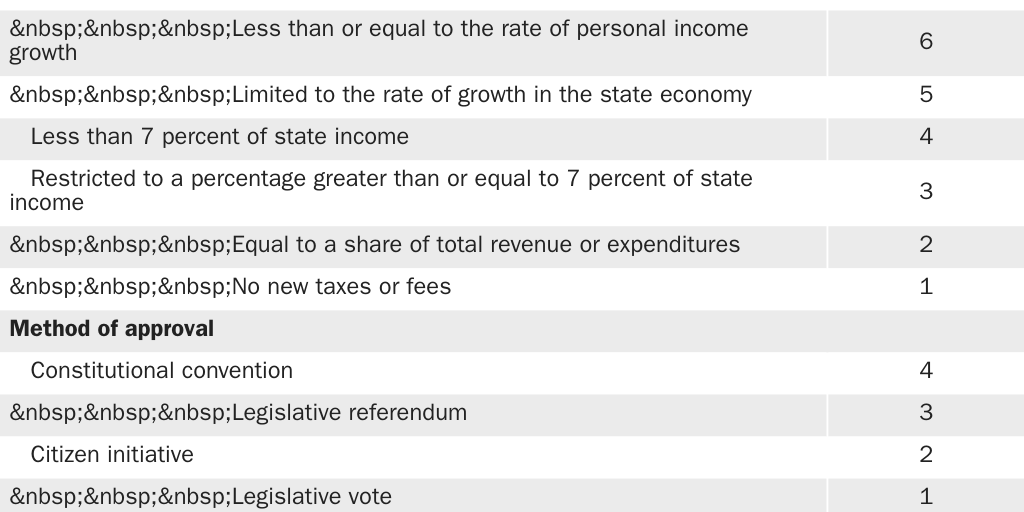
University of Wisconsin–Madison professor Lindsay Amiel and colleagues proposed a more complex stringency index in a 2009 paper, assigning a variable number of points to TELs based on numerous characteristics, as shown in Table 2.⁶⁰

Applying this index to state data from 1996 to 2011, Natalia Ermasova and J. M. Kulik found no association between TEL stringency and overall general fund spending.⁶¹ While they found that more stringent TELs were correlated with less spending on education, these savings were offset by greater spending on corrections and government administration.

The libertarian approach to state finance seeks to minimize taxation by eliminating unnecessary programs and privatizing those that remain. In this section, however, it is assumed that the size and scope of state governments will remain largely unchanged over the near term. Instead, recommendations are offered to minimize state governments’ economic impact, given their current scope.

As discussed in the revenue source section, high marginal tax rates increase budget volatility and contribute to out‐​migration. To avoid these problems, states should limit their highest marginal income tax rates and rely more heavily on consumption taxes.

States should continue the positive trend toward higher rainy day fund balances and other reserves. These funds can protect states from layoffs and service cuts during recessions or other contingencies.

Healthy reserves are especially important for states facing higher revenue volatility due to high marginal income tax rates, reliance on severance taxes, or dependence on tourism‐​related revenue sources.

Cash reserves can also be used to finance infrastructure rather than bond proceeds. With higher interest rates in 2022 and 2023, bonds have ceased to be an inexpensive form of financing. Going forward, additional bond issuance could burden the general fund with debt service costs, crowding out other priorities.

In many states, pension benefits for current employees are protected by law, so options for reducing unfunded pension liabilities may be limited. States should use surplus revenues to make additional pension fund contributions. They should also review actuarial assumptions, such as the assumed rate of return on pension fund assets, to ensure that they are realistic. While adopting more conservative assumptions will necessitate increased contributions in the near term, it will reduce the risk of unfunded liabilities spiking in future years.

It may be easier for states to focus instead on retiree health care obligations, which are less likely to have legal protections. Most public sector retirees are eligible for either Medicare or subsidized plans on their state’s health insurance exchange. To the extent that state policymakers deem retiree health benefits necessary, these benefits should supplement, rather than displace, federally provided coverage.

The best way to provide retiree health coverage without incurring unfunded liabilities is to offer health savings accounts. Employees can contribute to these accounts on a tax‐​deferred basis; retirees can later draw on the account to pay health insurance premiums without incurring a tax liability. Employees who leave an employer that offers retiree health savings accounts can retain their balances, whereas they risk losing defined post‐​employment benefits if they leave their jobs prior to those benefits vesting. So, health savings accounts are beneficial to employees regardless of whether employers match their contributions.

Transit and intercity rail projects often cost more and take longer to complete than originally estimated. Furthermore, they may fail to generate projected ridership, especially in the post‐​pandemic era. Transportation agencies, contractors, and advocates all have incentives to underestimate the costs and exaggerate the benefits of new infrastructure. Consequently, it is essential for state policymakers to seek input from independent, disinterested experts before committing state funds to these initiatives.

Any cost‐​benefit analysis should also consider the long‐​term costs of maintaining stations, track, equipment, and other system components. If fare revenues are unable to cover daily operations, let alone maintenance and retiree benefits, then alternative revenue sources must be found. If this alternative source is state general revenues or gas taxes, state policymakers should recognize that they will be diverting scarce funds to transit subsidies well beyond their time in office.

Most new routes can be serviced more cost‐​effectively by bus rapid transit or conventional buses than by rail. Buses benefit from standardization that often eludes rail systems, which frequently have custom components since different metro systems have different specifications for their rolling stock.⁶² When an agency attempts to construct or operate unique infrastructure, it loses the opportunity to benefit from the experience of other agencies, operators, and manufacturers. This may be one reason that the transit authorities of Boston, New York City, Washington, and the San Francisco Bay Area have all experienced problems with recent orders of rail cars.⁶³

Although major road projects may have more predictable costs and utilization than rail, they also create an ongoing maintenance burden. New projects should generally rely on toll revenues to cover life‐​cycle costs rather than on declining gasoline tax revenues. New bridges and highways should use dynamic tolling to better distribute utilization between peak and off‐​peak hours and to encourage commuters to share rides. To further reduce taxpayer risks, toll roads and bridges should be privately operated where possible.

Dynamic tolling and congestion pricing may also be applied to existing highways and urban streets to raise revenue for road maintenance and more evenly distribute traffic across the day.

As discussed earlier, the long‐​term educational benefits of state‐​funded public preschool programs are questionable at best. Although districts may be tempted to offset declining K–12 enrollment by adding programs for younger children, state policymakers should avoid funding these initiatives. If lawmakers insist on subsidizing childcare and early education, it is best done through vouchers. Cash subsidies are preferable to public provision because the latter can generate unfunded liabilities (especially pension liabilities) for future taxpayers.

K–12 public school districts, community colleges, and state universities should right‐​size the number of their staff and facilities to meet current and projected enrollment. If enrollment is falling, attrition and layoffs may be necessary. Staff reductions should not be limited to teachers, but rather should focus on administrative staff that may not be creating value for students. Policymakers should consider merging schools, and even colleges, to eliminate redundant administrative costs and free up additional real estate.

States should permit and encourage local education authorities and state educational institutions to sell surplus buildings, both to lower ongoing maintenance costs and to obtain one‐​time revenues. Aside from these financial considerations, educational institutions selling off spare buildings can potentially add to the community’s residential housing stock.

As of late 2023, state fiscal conditions have remained relatively strong, albeit with notable exceptions in California and New York. States with lower taxes and spending are better positioned to withstand a possible recession. They have also benefited from interstate migration as more people retire or work remotely. High‐​tax states should assess whether their residents are getting value for their money. While there is a constituency for ambitious government in high‐​tax states, other residents are concluding that the extra expense does not necessarily translate into better services or a higher quality of life.

This appendix addresses the question of whether more state spending necessarily translates into better outcomes for Medicaid, K–12 education, and higher education.

This section takes into consideration the relationship between Medicaid spending per adult beneficiary and attempts to correlate spending levels with each state’s death rate for individuals below the age of 65. Deaths among seniors are excluded because their primary health coverage is provided by the federal Medicare program.

Increasing Medicaid funding does not seem to be a good way to improve a state’s health outcomes. Figure 1 shows that there is a relatively poor correlation between increased Medicaid spending per adult beneficiary and death rates per 100,000 residents (the crude death rate) for ages 0–64. Although the trend line implies a slight decrease in crude death rates with increased adult Medicaid spending, this trend line does not fit the data especially well.

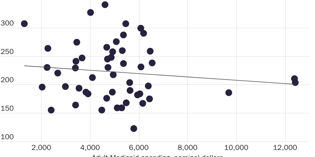
Moreover, states with comparable Medicaid spending per beneficiary may have large variations in crude death rates. For example, Utah and Vermont spent $5,794 and $5,465, respectively, per adult Medicaid beneficiary in 2019. However, Vermont’s crude death rate was 307, which is three times higher than Utah’s crude death rate of 123.

This observation is supported by extensive literature on the effects of state‐​provided welfare programs on health outcomes. A landmark experiment in Oregon, for example, showed that providing Medicaid merely increased the utilization of medical resources, but not health outcomes.⁶⁴ The well‐​known 1982 RAND Health Insurance Experiment also showed that a no‐​cost sharing medical plan merely increased utilization without improving outcomes.⁶⁵

The conclusion of the RAND Health Insurance Experiment has been confirmed by subsequent studies. For instance, a 1989 study by the Group Health Cooperative of Puget Sound found that “the introduction of a $5 copayment for office visits resulted in an estimated 10.9% decrease in primary care visits” (although it did not examine health outcomes specifically).⁶⁶ In Columbia professor Michael Eichner’s 1997 paper on the elasticity of health insurance, he also found that an approximately $2 increase in coinsurance reduced health care visits by one.⁶⁷ A 2001 article by researchers at the University of California, Los Angeles, found that “in a chronically ill population, cost sharing reduced the use of care for both minor and serious symptoms,” and noted that “no differences in self‐​reported health status were observed.”⁶⁸

If greater spending on schools improves learning outcomes, there should be a correlation between spending levels and standardized test scores. But an analysis of recent data does not show a statistically significant relationship between the two variables.

In November 2022, the US Department of Education released National Assessment of Educational Progress (NAEP) scores by state.⁶⁹ Four of those scores are available, covering reading and mathematics for fourth and eighth graders. Summing up these scores, which are all on a 0–250 scale, provides an overall picture of student educational achievement by state.

A regression analysis by the Census Bureau of 2020 K–12 public school finance data using this composite as the dependent variable, and current per pupil spending for each state as the independent variable, shows no statistically significant relationship at the 95 percent confidence level.⁷⁰

By contrast, the percentage of students eligible for free or reduced‐​price lunch is strongly related to test scores at the same confidence level. In a multivariate analysis by the National Center for Education Statistics employing both spending and free and reduced‐​price lunch data during 2019–2020 as independent variables, only the latter has a statistically significant coefficient.⁷¹

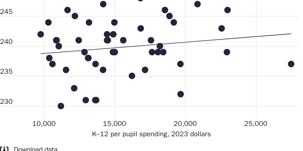
Figure 2 shows that increased K–12 per capita spending does not correspond to increased K–12 test scores. For example, Florida, which spends $11,671 per capita on K–12 education, has a relatively high fourth‐​grade mean math score of 246, while Alaska, which spends $19,677 per capita on K–12 education, has a mean fourth‐​grade math score of 232. (However, this graph does not show a causal relationship; increased K–12 per capita spending in some cases may be a response to low standardized test scores in prior years).

It could be expected that greater state spending on higher education would result in higher completion rates, as students respond favorably to better‐​funded educational offerings.

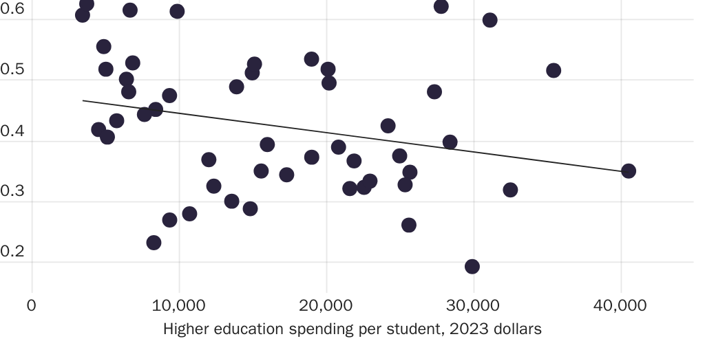
But as Figure 3 shows, there is a declining linear relationship between higher education spending per student and first‐​time four‐​year graduation rates for public colleges for the class of 2021. Vermont, for example, spent $3,754 per student on higher education in 2017 and had a public‐​school graduation rate of 63 percent four years later. On the other hand, New Mexico spent $25,649 per student on higher education in 2017 and had a 2021 first‐​time four‐​year graduation rate of 26 percent. Of course, the causal chain is not clear‐​cut: increased current per student higher education spending might be a result of low first‐​time four‐​year graduation rates in past years. However, higher education spending per capita does not seem to correlate with higher first‐​time four‐​year graduation rates for public colleges.

Joffe, Marc. “State Fiscal Health and Cost–Saving Strategies,” Policy Analysis no. 969, Cato Institute, Washington, DC, February 20, 2024.