
The health benefits of reducing fine particulate matter (PM2.5) anchor Environmental Protection Agency (EPA) air quality regulations and underpin the justification for a broad range of federal policies. Estimates of reduced adult mortality, in particular, drive these regulations, as seen in the Biden administration’s recent lowering of the National Ambient Air Quality Standard for PM2.5. Yet the link between PM2.5 and mortality remains uncertain and is subject to statistical weaknesses. The EPA’s cost-benefit analyses for PM2.5 standards tout large benefits against modest costs but overlook deeper ambiguities and geographic disparities. The EPA’s process for setting air quality standards should address all forms of uncertainty and explicitly weigh the costs involved. Devolving responsibility for air quality regulation to the states may offer opportunities to reduce complexity, tailor policies to local needs, and motivate innovative approaches, while a federal focus on interstate pollution could better reconcile health and economic considerations.
Introduction
When reading through federal regulatory notices and cost-benefit analyses, a common thread emerges: The health benefits of reducing emissions of particulate matter—small particles and droplets suspended in air—play a pivotal role in justifying many regulations, especially those from the Environmental Protection Agency (EPA) and the Department of Energy. In the last year of the Biden administration, several major regulatory actions, from limiting vehicle emissions to imposing energy efficiency standards on refrigerators and washing machines, were at least partly substantiated on the assumed health benefits of reductions in particulate pollution.1
Viewed collectively, these benefits make up a significant part of the justification for the entire regulatory state. From 2006 to 2016, the Office of Management and Budget reported that EPA regulations accounted for at least 71 percent of the total monetized benefits and 55 percent of the total monetized costs of all major federal regulations. Air quality rules specifically made up 95 percent of the total benefits of EPA regulations.2 Most of these benefits stem from estimated reductions in mortality caused by lowering emissions of fine particulate matter (particulates measuring less than 2.5 micrometers in diameter, or about 30 times smaller than a human hair, which are known as PM2.5).3 In some cases, such as the Mercury and Air Toxics Standards, more than 99 percent of the stated benefits came from the “cobenefit” of PM2.5 reductions, even though these were secondary to the regulation’s primary aim.4
PM2.5 is a regulatory category that refers to a mix of chemicals and substances emitted by a range of man-made and natural sources, including vehicles, restaurants, factories, power plants, wildfires, windblown dust, and vegetation. These particulates are thought to penetrate deep into the lungs and bloodstream, potentially causing significant health issues. In the short term, they may aggravate asthma, decrease lung function, and cause difficulty breathing. In the long term, they may create chronic health problems.
As a result, particulate matter, including PM2.5, is regulated as one of six “criteria” air pollutants under the Clean Air Act (CAA), with the National Ambient Air Quality Standards (NAAQS) setting a permissible exposure level across the United States. Most recently, the Biden administration lowered the PM2.5 standard from 12 to 9 micrograms per cubic meter of air (μg/m³). As with earlier reductions in the PM2.5 NAAQS, and the use of PM2.5 benefits in other air quality regulations, this decision was based on scientific evidence suggesting a link between PM2.5 exposure and mortality.
However, since particulate matter was first monitored and regulated there has been considerable disagreement about its actual health effects. While the EPA and many epidemiologists consider the issue resolved, others question the scientific evidence.
After decades of contentious and highly politicized debate, PM2.5’s health effects remain a divisive issue. The root of the dispute lies in the structure of the NAAQS itself and the role that science plays in the policy process.
We propose reforming the NAAQS with three key goals in mind:
- Incorporating all sources of uncertainty, including unanswered questions about the causal relationship between particulate matter and long-term mortality and the form of that relationship.
- Requiring consideration of regulatory costs. The EPA is currently precluded from considering any factors beyond health risks when determining the permissible level of PM2.5. This has created a policy process that obscures the tradeoffs involved and excludes additional normative questions, including the economic consequences of tightening PM2.5 emissions standards.
- Transferring responsibility for deciding permissible PM2.5 exposure levels to the states. While the federal government can play a legitimate role in regulating interstate pollution, shifting the responsibility for determining ambient air quality to state governments will create opportunities to decrease administrative complexity and encourage more localized, flexible approaches.
For some people, particularly those who experienced the air pollution of the 1950s and 1960s, federal leadership in air quality regulation may be viewed as a necessity. The CAA and national air quality standards are often seen as a natural response to an environmental crisis. But after half a century of improving air quality, the context is now very different from when federal involvement in pollution regulation began. It is important to reassess whether the measures that once seemed essential continue to serve the best interests of public health and economic efficiency.
The Clean Air Act and the National Ambient Air Quality Standards
Today it is hard to fathom the extreme level of air pollution in the United States that set the stage for the CAA. In the late 19th and early 20th centuries, American cities experienced soot, dust, acidic particles, and gas emissions that were sometimes so severe that they blocked sunlight.5 In Pittsburgh, streetlights were at times kept on past 10 a.m.6 The intense pollution from coal burning and steel production earned Pittsburgh the nickname the “Smoky City.”7
Initially, problems with air pollution were addressed through private litigation under nuisance and trespass laws.8 By the late 1800s, local governments had enacted measures to control pollution. Municipal ordinances and a shift from coal to electrification and natural gas had mixed success in reducing pollution.9
Major events in the 1940s and 1950s drew attention to air pollution and its potential health effects. Los Angeles experienced its first smog event in 1943. Without a known source, many assumed that the noxious fog blanketing the city, burning residents’ eyes and reducing visibility, was a Japanese gas attack.10 It wasn’t until the early 1950s that scientists learned the smog was caused by refinery and automobile emissions trapped in the Los Angeles Basin and irradiated by the California sun, thus creating high levels of ozone.
In 1948, Donora, Pennsylvania, a small town about 20 miles outside of Pittsburgh, experienced a tragic pollution event. A temperature inversion—a meteorological phenomenon where cold air is trapped at the ground beneath a layer of warm air—created a multiple-day buildup of sulfurous emissions from the town’s steel and zinc smelters. The extreme level of pollution sickened nearly 6,000 people (about half the town’s working population), and 20 people died.11 Similar disasters occurred in London during the 1950s, most notably the infamous “Great Smog of 1952,” when 4,000 people died over four days from extreme pollution.12
These disasters heightened public concern and, in 1955, President Dwight D. Eisenhower signed the Air Pollution Control Act, which funded federal research on air pollution and provided technical assistance to the states.13 However, public unease over air pollution continued to grow, especially after the publication of conservationist Rachel Carson’s book Silent Spring, and pressure for stronger federal action increased.14 The Clean Air Act of 1963 created federal grants to help develop state and local pollution-control programs and established a procedure to address problems of interstate pollution, but it still left most authority with state and local governments.15
Those governments demonstrated little interest in utilizing the processes established by the new law. By the end of 1967, the Department of Health, Education, and Welfare (HEW) had no requests for help with addressing pollution within the states and only three requests for help with interstate pollution.16 In Congress, though, there was still support for a federal response to air pollution, which led to the Air Quality Act of 1967.
Debates arose over the merits of two approaches to air pollution control: emissions standards and ambient air quality standards. Emissions standards set limits on how much pollution a source can emit, based on the assumption that a practical degree of control is achievable.17 In contrast, ambient air quality standards, or “risk-based standards,” directly consider the health risks associated with differing levels of outdoor air pollution. These standards define the acceptable amount of pollution based on minimizing health risks, and areas exceeding these levels must enact pollution-reduction strategies.
The benefit of emissions standards is that they are relatively easy to implement and enforce; the downside is that they can be inflexible and costly.18 In contrast, ambient air quality standards are complex and require knowledge of the health effects of pollution to determine an appropriate permissible level of emissions. Once established, however, they allow different jurisdictions to determine the most effective methods of emissions reduction.
Another important question was whether these standards should be applied nationally or tailored to regional conditions. Advocates for national standards argued that without uniformity, industries in areas with weaker regulations would have an unfair competitive advantage over those in stricter regions.19 Critics argued that local conditions vary, and a one-size-fits-all approach would result in overregulation in some areas and underregulation in others.20
Ultimately, the 1967 act avoided setting national standards. It required HEW to establish air quality control regions and develop criteria about the health risks of air pollution and the costs and effectiveness of different control technologies. States were then required to develop plans to establish air quality standards and implement control strategies, which would be approved by HEW.21 Progress in addressing pollution was slow and HEW’s delayed creation of air quality control regions and promulgation of the criteria for setting pollution standards meant that by 1970 only 23 states had submitted implementation plans, and none had received federal approval.22
In the meantime, environmentalism became an important part of President Richard Nixon’s political agenda.23 In his 1970 State of the Union Address, to position himself ahead of potential rivals in the 1972 election, he promised an expansive environmental program that would “be the most comprehensive and costly program in this field in America’s history.”24 The result was the Clean Air Amendments of 1970, which created national emissions standards for new major stationary sources of pollution, directed the newly formed EPA to set national ambient air quality standards, and mandated lower automobile emissions.
Initially, the NAAQS were applied to five “criteria” air pollutants, including sulfur oxides, nitrogen oxides, and particulate matter (at that time this referred to suspended particles up to 100 micrometers, measured as total suspended particulates [TSP]). The EPA was tasked with developing “air quality criteria” that would “reflect the latest scientific knowledge useful in indicating the kind and extent of all identifiable effects on public health or welfare which may be expected from the presence of such pollutant in the ambient air, in varying quantities.”25 The EPA would then set two types of standards, a primary standard to “protect the public health” and a secondary standard to “protect the public welfare,” such as against damage to agriculture or reduced visibility.26 States then had to submit plans for achieving these standards.
Since 1970, the CAA and NAAQS have been revised several times, most notably through extensive amendments in 1977 and 1990. In the mid-1980s, the measurement of particulate matter was changed from the broader category of TSPs to particulates less than 10 micrometers in diameter (PM10). In 1997, separate standards for PM2.5 were added, including an annual standard and a 24-hour standard.
During this time, the CAA and NAAQS faced numerous legal challenges. One significant 2001 Supreme Court case (Whitman v. American Trucking Associations, Inc.) addressed, among other issues, whether the EPA could consider the costs of reducing pollution when setting NAAQS. Then-EPA administrator Carol Browner argued that the CAA specifically does not allow the EPA to account for costs when determining air quality standards, instead requiring that “pollution limits be based solely on health, risk, exposure and damage to the environment, as determined by the best available science.”27 The Supreme Court ruled unanimously in favor of the EPA, affirming that the Clean Air Act does not allow cost considerations in setting air quality standards.28
Over the past century, air quality in the United States has improved substantially, though it is still debated whether the credit goes to the CAA and NAAQS or to preexisting downward trends.29 In 1960, for example, the annual average TSP concentration in both Los Angeles and Pittsburgh was 143 μg/m³.30 By 1986, the final year before PM10 became the standard, TSP levels had fallen to 101 μg/m³ in Los Angeles and 55 μg/m³ in Pittsburgh—declines of 29 and 62 percent, respectively.31 Since 1990, national annual average PM10 levels have declined by 29 percent, and since 2000, average PM2.5 levels have declined by 37 percent.32
In the context of the high day-to-day levels of pollution experienced in cities across the United States, and with the concern generated by pollution disasters such as the London Great Smog of 1952, where daily levels of TSPs were at times more than 1,600 μg/m³, the first federal interventions in air pollution in the 1950s and 1960s may have been warranted.33 The question today, after decades of improving air quality, is whether further efforts at nationwide incremental improvements are worthwhile.
Given that cost considerations are precluded from the NAAQS process, the calculation of the appropriate level of ambient pollution is based entirely on “scientific knowledge.” This has created a highly politicized process and a contentious debate over the scientific evidence of the health effects of particulate matter.
The Limits of “Scientific Knowledge”
The fundamental problem in the debate about the effects of particulate matter on health is the difficulty in proving that long-term exposure to PM2.5 causes mortality. The ideal scientific method to establish a causal relationship between PM2.5 exposure and health outcomes would be a randomized controlled trial in which participants are randomly assigned to different exposure levels. Random assignment ensures that all other potential causes of health outcomes, such as age, preexisting health conditions, or smoking history, are not correlated with exposure to particulates in the air. If the number of participants is sufficiently large, researchers would be confident that any differences in health outcomes between the exposed and unexposed groups are caused by the differences in PM2.5 exposure.
Substantial obstacles make such a trial impractical.34 Instead, epidemiology uses statistical methods to analyze nonexperimental observations of people’s natural exposure to air pollution and their health outcomes, attempting to mimic the conditions of a trial. However, all statistical analyses imperfectly replicate experiments.
This statistical imperfection, combined with the legal requirement that the standard-setting process consider the latest scientific knowledge, has resulted in a decades-long debate about the results of observational studies. Many epidemiologists—and the EPA—contend that the weight of the evidence shows a correlation between PM2.5 and mortality; thus, particulate matter causes deaths.35 Other scholars argue that epidemiological findings of correlation provide insufficient evidence that the relationship is causal.36
Historical Studies on PM2.5 and Mortality
Historically, the EPA has relied on the Harvard Six Cities Study (SCS) and the American Cancer Society study (ACS) for its estimates of mortality effects of particulate matter. First published in 1993, the SCS examined about 8,111 people living in six American cities that were chosen to represent a range of pollution levels.37 The ACS study, initially published in 1994, followed more than 550,000 people in 151 US metropolitan areas.38 Both studies found an association between PM2.5 and mortality, and both have had follow-up studies supporting their results.
They have also faced considerable scrutiny. Critics question whether these studies adequately controlled for alternative factors (called “confounding variables” by epidemiologists) that, if included, would eliminate or severely attenuate the effect of PM2.5 exposure on mortality. In statistical terms, exclusion of such factors may introduce bias: systematic errors that cause the estimates to deviate from the true value. Sedentary lifestyles or smoking, for example, rather than PM2.5 exposure, might explain the SCS and ACS findings.39 Failing to account for these factors could lead to biased results, overestimating or falsely suggesting an association between PM2.5 and mortality.
The Health Effects Institute, a reputable independent organization jointly funded by the worldwide automotive industry and by the EPA, conducted a reanalysis of the studies, finding biologically puzzling results.40 The SCS found increased mortality in men but not in women.41 The ACS found increased mortality for moderate exercisers but no effect for those who did not exercise or who were heavy exercisers.42 And both studies found increased mortality in people with less than a high school education but not more.43
Those results suggest some factor other than PM2.5 may be responsible. For example, suppose that whether someone completed high school is linked to another factor influencing both exposure to particulate matter and mortality: socioeconomic status. Socioeconomic status affects the likelihood of living in areas with higher pollution levels and access to health care. The observed association between particulate matter and mortality might be explained by differences in socioeconomic status. However, in the absence of measures of socioeconomic status, the empirical analysis attributes increased mortality to PM2.5 exposure. Including educational attainment, for example, partially controls for socioeconomic status and may reduce the observed effect of PM2.5.
The Health Effects Institute also considered the effects of migration. After adjusting for population change in the ACS, the reanalysis found that PM2.5 had no effect on mortality. Around 18.5 percent of the SCS subjects moved from their original city, and they were, on average, younger and more highly educated than the subjects who didn’t move.44 The reanalysis concluded that the SCS mover group had a lower relative risk than nonmovers and that the estimates of the PM2.5 effects on their mortality were not statistically different from zero.45
These results suggest the existence of selection effects in the data. Cities with population declines in the 1980s were Rust Belt cities with higher particulate matter levels. As younger, better educated people moved away, the remaining population may have had relatively higher mortality rates. It is possible that if the migrants had stayed, the observed PM2.5 effect would have been attenuated.
Unmeasured confounding and selection effects have led some critics to conclude that the statistical association the SCS and ACS identify between particulate matter and mortality is not sufficient to prove that PM2.5 causes death. In a 2008 survey of a dozen experts, including three authors of the ACS and SCS, respondents were asked whether the relationship between PM2.5 and mortality was causal. Four experts assigned a 10 to 65 percent probability to the relationship not being causal, three said there is a 5 percent probability, and five said there is a 0 to 2 percent probability. Applying a typical 95 percent confidence standard implies that seven of the experts would not reject the hypothesis that PM2.5 does not cause mortality.46
Recent Particulate Matter Epidemiology
New research attempts to address the concerns that traditional statistical methods do not establish a causal relationship. In a 2020 paper, Xiao Wu and colleagues studied Medicare enrollees, using two traditional approaches and three generalized propensity score models to assess the relationship between PM2.5 and mortality. Based largely on their generalized propensity score methods, the authors argue that their study “provides the most robust … evidence to date on the causal link between PM2.5 … and mortality among Medicare enrollees.”47
Generalized propensity score methods attempt to duplicate the randomization of a controlled trial. They do this by ensuring that measured confounding variables, such as smoking, are identical across different levels of PM2.5 exposure. By comparing cases with similar values of control variables but differing exposure to PM2.5, a study can estimate the effect of PM2.5 on mortality while controlling for other factors. However, questions about Wu’s methodology and reasons to be skeptical of their findings of a causal relationship remain.
Measurement Issues
Empirical work is only as good as the data that are used. And data are often less than ideal. Researchers make methodological choices to deal with imperfect data, and these decisions affect their results.
In general, the larger the number of data points in a statistical analysis, the smaller the confidence levels that surround the results and the greater the likelihood that the results are “real” and “different from zero.” Wu stresses that their analysis uses “the largest air pollution study cohort to date … more than 68.5 million Medicare enrollees (65 years of age or older) from 2000 to 2016, including demographic information on age, sex, race/ethnicity, date of death, and residential ZIP code.”48
The emphasis on the number of Medicare enrollees, however, is misleading. Their analysis aggregates annual deaths at the zip code level, estimating mortality effects based on zip code exposure levels and demographic variables. The number of zip codes included is large, and thus their sample size is still large, but it is not 68.5 million—it is only 532,729 (i.e., 31,337 zip codes over 17 years).
In addition, the analysis uses zip-code aggregates rather than the individual-level data. And using aggregate data to make inferences about individuals is so problematic that it has its own term in the literature: ecological fallacy.49 The propensity scores estimated in Wu’s analysis are not propensity scores for individuals, but instead, they are the propensities for a zip code. The study does not measure individual exposure to PM2.5, nor does it include information about individual health, behavioral, or socioeconomic factors.
Excluding meteorological variables, the control variables are obtained from two sources. Demographic and economic information (which includes, for each zip code, the population density, percent below poverty level, percent Hispanic, percent black, percent below high school education, percent owner-occupied housing, median household income, and median home value) come from the Census Bureau’s American Community Survey five-year estimates. Smoking rate and mean body mass index (BMI) are county-level estimates from the Centers for Disease Control and Prevention’s Behavioral Risk Factor Surveillance Survey (BRFSS). The survey’s data for smoking and BMI are only available at the county level. Wu applies the county-level estimate to all the zip codes in that county. This exacerbates the ecological issues of using zip code data to represent individuals.
Both the census and BRFSS data have measurement error because they are surveys. This survey measurement error is not incorporated into Wu’s analysis, thus reducing the precision of estimates and potentially introducing bias if the survey errors are correlated with exposure and mortality. A study of survey measurement error of the American Community Survey found that methods that ignore the error were biased, and they underestimated the uncertainty of the estimates.50
Wu not only uses aggregate data to make inferences about individuals, they also use rolling averages as if they were individual year estimates. Against the specific recommendations of the Census Bureau, they use overlapping data from the American Community Survey. At smaller geographic levels, such as zip codes, single-year point estimates are not available.51 Instead, the census releases five-year rolling estimates. For example, the 2007–2011 five-year estimate of median household income for a zip code includes estimates from all five years that are pooled, weighted, and processed to calculate a single estimate. But this estimate does not represent the median income for a single year, but rather for all five years. Comparing estimates from 2007–2011 and 2008–2012 means that four of the five years of data are overlapping, and “the Census Bureau strongly recommends against comparing estimates in overlapping five-year periods since much of the data in each estimate are the same.”52 Wu , however, uses the five-year estimates to compare data between subsequent years (with 2007–2011 data used for 2011, 2008–2012 data used for 2012, and so on to 2016).
This use of the pooled estimates smooths the data relative to its true variability. Thus, the confidence interval surrounding the estimated effect of PM2.5 is larger than estimated, increasing the risk of a false positive result.53
Finally, a large portion of the data used by Wu is imputed. Many zip codes lack data for multiple years. The American Community Survey data at the zip code level starts in 2011 (i.e., five-year estimates for 2007–2011). Wu uses decennial census data for 2000 and interpolates for 2001–2010. The BRFSS data end in 2012, with missing data for many counties before that. The authors extrapolate for 2013–2016 and interpolate missing data for earlier years, when necessary, and they use a moving average to interpolate their data so that each imputed data point is based on the most recent existing data. This reduces the variability of the data and creates a false sense of precision in the statistical estimates.54
If the missing data are correlated with particulate matter levels and mortality, imputation results in biased estimates.55 For example, the number of years of missing BRFSS data is correlated with the population density of a zip code. The roughly 53 percent of zip codes with only four years of missing data (the minimum amount, since there is no BRFSS data for 2013–2016) have a median population density of 1,048 people per square mile, whereas zip codes with five or more years of missing data have a median population density of 58 people per square mile.56 Thus, the data for rural zip codes is more likely to have higher levels of interpolation.
Questions about imputed missing values or measurement error are common in statistical analyses. However, the scale of these questions in Wu’s analysis is noteworthy, as most of the control variables used are largely imputed. All told, only 2 years (2011 and 2012) have nearly complete data. The other 15 years used in the analysis rely on either imputed census data (interpolated based on misused five-year estimates) or BRFSS data (with county-level data assigned to each zip code) or both.
Thus, the authors’ statistical tests, which purportedly rely on 17 years’ worth of data to demonstrate a causal relationship between PM2.5 and mortality, actually depend on far fewer years of problematic data for many key factors.
Unmeasured Confounding
Econometric analysis of the effect of particulate matter on mortality must control for factors that are correlated with both exposure and mortality. Failure to include these factors, referred to as confounders in the epidemiological literature, results in biased estimates of the effect of PM2.5 on mortality. Some of these, such as age and sex, are easily measured and included.
Other factors are measured with less precision. For example, in Wu’s analysis the smoking rate variable is the percentage of people in a county who have ever smoked. This omits information that affects mortality, including smoking intensity, duration of smoking, and time since cessation. Including a coarse variable like “ever smoked” versus “never smoked” may account for some of the smoking-related confounding. But residual confounding may remain if the smoking risk factors that were omitted differ between high and low PM2.5 areas.57
The generalized propensity score methods used by Wu do not require assumptions about the form of the relationships between PM2.5 and the control variables. By balancing the measured confounders across propensities to be exposed to PM2.5 they can isolate the mortality effects of PM2.5 from the effects of the included alternatives. However, generalized propensity score methods still rely on the assumption that there is no unmeasured confounding. A randomized controlled trial can demonstrate a causal link because by randomly assigning subjects to exposure and nonexposure groups it ensures that, on average, both measured and unmeasured confounding variables are evenly distributed. An observational study using generalized propensity score can only ensure that measured confounders are evenly distributed.58
Past research has explored various potential unmeasured confounders, such as occupational history, health care quality and access, preexisting health conditions, physical activity, diet, noise pollution, and stress levels.59 If these or other confounders are correlated with PM2.5 exposure and mortality, their exclusion suggests that the estimated effect of PM2.5 on mortality is too large or, if the omitted confounding relationship is strong enough, nonexistent.
Previous evidence does suggest that unmeasured confounding exists in assessments of PM2.5 and mortality. A notable example is demonstrated in a 2011 study by Sonja Greven and colleagues that separates trends in PM2.5 into two parts: a “global” trend that measures changes in PM2.5 on a national level and a “local” trend that measures PM2.5 at a local level.60 If a relationship between declining PM2.5 and improving life expectancy is observed on a national scale, the same should be observed at a local level. Cities with sharper declines in particulate matter should see larger increases in life expectancy. Greven, however, finds that while there is a national association between PM2.5 and life expectancy, there is no such relationship on a local level.
This result could indicate the presence of a national confounder that is biasing the global analysis. Although alternative explanations have been proposed, economists Wonjun Chang and colleagues use simulations in their study to show that the likely reason is a time-varying, unmeasured, confounding variable that is associated with long-term trends in both PM2.5 levels and mortality.61 If this is correct, it would mean that there is no real causal relationship between PM2.5 and mortality.
Selection Effects
Selection effects arise if the “choice” to be exposed to low or high levels of PM2.5 is not random. Selection creates bias in causal estimates if the “choice” to be exposed is correlated with other causes of mortality.
One important critique of previous air pollution epidemiology was that the ACS and SCS studies did not account for migration. If people who moved away from cities with high PM2.5 levels (generally those who were younger and better educated) had not moved, the observed effect of particulate matter may have been smaller.
Wu’s study also does not consider the effects of migration, and thus relies on the assumption that people living in areas with high and low levels of PM2.5 are, on average, identical after controlling for the area-level covariates. But if people select into high- and low-pollution areas based on characteristics that are related to mortality, then this assumption is incorrect.
Census Bureau migration data do indicate that, on average, people aged 65 and over move from high PM2.5 to low PM2.5 areas. To illustrate this, we link American Community Survey 2011–2015 estimates of county-to-county migration flows to Wu’s estimates of PM2.5 levels in 2015.62 On average, annually about 17 people aged 65 and over moved from a county above the median level of PM2.5 (roughly 7.8 μg/m³), while about 19 people aged 65 and older moved to a county below the median level. Expanding the analysis to people aged 55 and over finds a per county annual flow of about 35 people from high to low PM2.5 counties.
In percentage terms, this flow is small: on net, high PM2.5 counties each lost about 0.1 percent and low PM2.5 counties each gained about 0.16 percent of people aged 65 and over annually. However, these are annual estimates. Assuming the 2011–2015 trend is true for the entire 16-year period of Wu’s, the cumulative number of movers is more substantial. And this type of migration bias can have substantial effects even when the number of people who move is small.63
Additionally, the localized effects in areas with extreme high or low levels of PM2.5 may be much higher. In Los Angeles County, which has high levels of particulate matter, for example, on net more than 6,000 people aged 65 and over (and nearly 15,000 people aged 55 and over) moved away annually. That is 0.51 percent of the total 65 and over population (and 0.65 percent of the 55 and over population). If this estimate is accurate for the full 2000–2016 period, this would mean that almost 9 percent of the 65-and-over population of the county moved elsewhere during Wu’s analysis.
Furthermore, because American Community Survey migration data is only available at the county-to-county level, this ignores people who move from high to low PM2.5 areas within a county. A more in-depth analysis that accounts for zip code to zip code migration might find an additional correlation between migration and PM2.5 levels.
The effects of migration only matter if the people who move and the people who remain are different. For example, if people who move to places with less air pollution live healthier lifestyles, are more active, have fewer preexisting health conditions, or are wealthier, then the difference in mortality rates between high and low PM2.5 areas may reflect these underlying differences rather than a causal relationship between particulate matter and mortality.
E‑Value
Wu’s primary measure of the robustness of their findings is their calculation of an “E‑value.” They define it as:
The E‑value for the [relative risk] … can be defined as the minimal strength of an association … that an unmeasured confounder would need to have with both the exposure and outcome, conditional on the covariates already included in the model, to fully explain the observed association under the null.64
In other words, the E‑value measures the relationship that an unmeasured confounder would need to have with both PM2.5 levels and mortality for the analysis actually to be estimating the effects of that confounder, implying that the true relationship between PM2.5 and mortality is zero. Wu finds an E‑value of 1.32, meaning that an unmeasured confounder must be both associated with a 32 percent higher likelihood of being exposed to 10 μg/m³ more of PM2.5 and a mortality rate 32 percent higher than the baseline for the confounder to fully explain away the effects of PM2.5.
At first, this estimated E‑value seems like strong evidence that there is unlikely to be an unmeasured confounder of the magnitude necessary to justify rejection of Wu’s findings. A few key caveats, however, suggest that some skepticism is still warranted.65
First, the estimated E‑value assumes that the unmeasured confounder nullifies the effect of PM2.5. If the true effect of particulate matter is less than they measure, but not zero, the necessary strength of the relationship of the confounder between exposure and outcome is smaller.
Second, the E‑value, as they describe it, suggests the necessity of a single strong confounding variable that alone explains away their entire findings. The E‑value simply measures the strength of association necessary for the estimated relationship between PM2.5 and mortality to be spurious, but it does not tell us whether one strong unmeasured variable is responsible for all of that bias or whether the bias stems from the combined effects of multiple weaker confounders.66
Third, the E‑value is the minimum strength of association between the unmeasured confounders and both exposure and outcome, assuming that the relationships with exposure and outcome are equal. A confounder with a stronger relationship to PM2.5 exposure but a weaker relationship with mortality (or vice versa) could still imply that the estimated PM2.5 effect is false.67 For example, if an unmeasured confounder is associated with a 100 percent higher likelihood of being exposed to 10 μg/m³ more PM2.5 (i.e., a person is twice as likely to be exposed to 10 μg/m³ more PM2.5, or 2.00 on a relative risk scale), it would only need to be associated with a 13 percent increase in mortality to nullify the observed effects (i.e., a relative risk of 1.13).
Finally, Wu reports their E‑value in terms of a 10 μg/m³ increase in PM2.5 exposure. While this is standard in PM2.5 epidemiology, it minimizes how large a difference 10 μg/m³ really is. Based on their PM2.5 data, 10 μg/m³ is larger than the range of particulate matter measured for the majority of zip codes. For example, in 2016, this difference corresponds to the range between the 0.02 and 99.98 percentiles of zip codes.68 The E‑value for a 1 μg/m³ increase is 1.08.69
Thus, while the E‑value does help quantify the residual bias necessary to suggest that the estimated effect of particulate matter on mortality is false, a more complete view of the E‑value qualifies Wu’s claims.
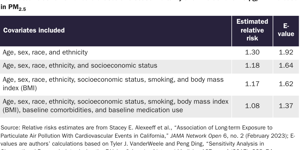
Simply viewing the E‑value as the strength of association necessary for one unmeasured confounder to nullify the results implies a much more difficult threshold to meet than when you consider the collective effect of many weaker confounders. This is illustrated by reviewing the results of a recent study on the effect of PM2.5 on cardiovascular health.70 As shown in Table 1, a model that includes only age, sex, and race and ethnicity as covariates finds a relative risk of cardiovascular disease mortality of 1.30 for a 10 μg/m³ increase in exposure. The E‑value of such a large relative risk is also large, 1.92, meaning that a single unmeasured confounding variable would need to be associated with a 92 percent higher likelihood of both being exposed to 10 μg/m³ and dying from cardiovascular disease. However, as additional confounders are included in the model, the relative risk and, therefore, the E‑value, quickly decrease. The full model, which additionally includes socioeconomic status, smoking, BMI, and baseline comorbidities and medication use, finds a relative risk of 1.08 and a much lower E‑value of 1.37. How might both the relative risk and the E‑value change if further variables were added, such as data on physical activity, nutrition, or more detailed smoking information?
The uncertainty of the Wu findings can be summarized with one question: Do unmeasured factors associated with both higher PM2.5 and higher mortality rates attenuate or eliminate the observed relationship between particulate matter exposure and mortality?
There are many unmeasured disparities between zip codes with large differences in PM2.5 levels. For example, zip code 90018 in the heart of Los Angeles, with a PM2.5 level of nearly 12 μg/m³ in 2016, was home to 50,000 people who lived in 3 square miles, as compared to zip code 98827 in northern Washington State with a PM2.5 level less than 2 μg/m³, where about 270 people were living in 320 square miles.71 We believe there is a strong possibility that some of the unmeasured differences between these areas account for variations in mortality.
Given that the propensity score methods used by Wu rely on imputed and misused data at the area level and cannot overcome unmeasured confounding variables or selection bias, their analysis does not resolve the PM2.5 debate.
Beyond Epidemiology: Quasi-Experimental Approaches in Environmental Economics
Economists also have examined the health effects of air pollution. These studies often use “natural” experiments—real-world events that create conditions similar to random assignment. In a 2009 paper, economists Michael Greenstone and Ted Gayer critique earlier nonexperimental studies, arguing that both the economic and health research on air pollution may suffer from biased results. They emphasize the importance of using quasi-experimental methods to draw more reliable conclusions. The propensity score methods used by Wu are also considered quasi-experimental but rely on observational characteristics to mimic randomization. In contrast, economists have utilized external sources of variation, such as policy changes, natural cut-offs, or events that create clear differences between treatment and control groups. In theory, such research designs yield unbiased estimates of the effects of pollution on health.
Short-Term Studies
Some studies use changes in wind direction as the equivalent of an experiment. Those who are downwind are more exposed to pollutants, while those who are upwind are less exposed. Changes in wind direction, by themselves, are assumed not to affect mortality. Thus, any change in mortality associated with changes in wind direction is a result of increased pollution exposure. Because wind changes are not long-term, such studies examine short- rather than long-term exposure effects on health.
In a 2019 paper, for example, Tatyana Deryugina and colleagues investigate the effects of PM2.5 changes on mortality.72 They estimate that a 1 μg/m³ increase in PM2.5 causes a 0.18 percent increase in three-day mortality rates for adults aged 65 or older. This is substantially smaller than Wu’s results, whose estimate that long-term exposure to 1 μg/m³ more PM2.5 increases elderly mortality by 0.64 percent.73
Some portion of the acute mortality effect is the result of “mortality displacement”—deaths among already frail people with short life expectancies. Deryugina argues that their results are not driven by mortality displacement because their estimated mortality effects increase over time—but the increase stops after only 14 days.74
In a 2023 analysis, Tatyana Deryugina and Julian Reif use similar estimates of the acute effects of air pollution to model long-term mortality.75 However, instead of PM2.5 they study the effects of sulfur dioxide exposure. They find that a 10 percent increase in sulfur dioxide causes a 0.33 percent increase in mortality for all ages. They then use a model of long-term human health to infer chronic effects based on the observed short-term effect. The model finds that a permanent decrease of 10 percent of sulfur dioxide pollution would increase life expectancy by 1.18 to 1.32 years. These long-term estimates are seven to eight times larger than the projections suggested by simple linear extrapolation of the short-term effects. Based on the amount of PM2.5 that is cotransported with sulfur dioxide, and the extreme assumption that all of the estimated health effects are caused by the cotransported PM2.5, Deryugina and Reif’s estimates would imply that a permanent 1 μg/m³ decrease in PM2.5 would increase life expectancy by 0.47 to 0.57 years.76
We believe that the chronic effects estimated by Deryugina and Reif should be viewed cautiously. Their model of long-term health is carefully calibrated and validated against real-world data, which suggests that it may be more accurate than simple linear extrapolation. But it is still a projection based on observations of mortality in a one-month window following one day of elevated exposure. The cumulative mortality effects of a one-day increase in exposure level off after only 35 days.77 And their estimates are based on observations of sulfur dioxide exposure, not PM2.5.
Long-Term Studies
In a 2020 study, Michael Anderson attempts to analyze the long-term mortality effects of pollution, although again, not specifically PM2.5 exposure.78 Anderson compares mortality differences between those people who are chronically upwind and downwind of major highways in Los Angeles, where winds flow from west to east off the ocean. He estimates that a doubling of time spent downwind increases mortality rates for people aged 75 or older by 3.8 to 6.5 percent. However, because PM2.5 concentrations decay to background levels within a relatively short distance of highways, these effects arise from exposure to ultrafine particles (particles with a diameter of 0.1 micrometer or less), nitric oxide, and carbon monoxide, rather than PM2.5.
Alan Barreca and colleagues exploit a difference in pollution controls on coal-burning power plants to evaluate how a change in sulfur dioxide affects long-term mortality.79 In the 1990s, the Acid Rain Program required only certain power plants to limit emissions, which created a permanent decrease in sulfur dioxide pollution. By comparing mortality before and after control technologies were installed in areas near the power plants, and then contrasting this trend with mortality rates in areas far from the regulated power plants that did not experience the same drop in pollution, Barreca isolates the mortality effects of sulfur dioxide. They find that the sulfur controls caused a statistically significant drop in cardiorespiratory-related deaths and that the effect was cumulative. While no reduction in mortality was detected immediately after the controls were implemented, the effect was detected 10 years later.
However, there are some puzzling results. When differentiating by age group, the authors found no effect for people under 35, the largest effect for people between 35 and 64, and a significant, but much smaller effect for people aged 65 and over. In 2005, for example, they estimated a 1.6 percent decrease in cardiorespiratory mortality for the middle-aged group and only 0.2 percent for the elderly group. Why is the estimated effect on people aged 65 and over so much smaller when elderly people are typically believed to be more sensitive to chronic air pollution exposure?
Barreca attempts a rough conversion of their sulfur dioxide estimates to PM2.5 mortality effects by modeling the relationship between PM2.5 levels and controls on sulfur emissions. Their approximate result is that a 1 μg/m³ decrease in PM2.5 causes a 1.1 percent decrease in the cardiorespiratory mortality rate for people aged 35–64.
China Coal-Use Studies
A series of studies exploits a policy discontinuity in China to estimate the effects of particulate pollution. From 1950 to 1980, the Chinese government provided free coal for winter heating in homes and offices in North China, demarcated by a boundary line formed by the Huai River and Qin Mountains, leading to a coal-burning heating infrastructure that does not exist in the south. As a result, pollution levels, as measured by total suspended particles (a category that includes PM2.5 and larger particles) and PM10 (which includes PM2.5 and particles up to 10 micrometers in diameter), remain much higher north of the Huai River than south of it. Assuming that the populations directly north and south of the river are otherwise similar, this discontinuity provides an opportunity to estimate the effect of particulate matter on mortality.
In a 2013 study by Yuyu Chen and colleagues, they find that, from 1981 to 2000, average TSP levels north of the river were approximately 552 μg/m³ compared to 355 μg/m3 south of the boundary.80 They estimate that a 100 μg/m³ increase in TSP reduced life expectancy at birth by about three years. In 2017, Avraham Ebenstein and colleagues analyzed PM10 levels from 2004 to 2012 and found average levels of about 120 μg/m³ north of the river and 91 μg/m³ south of the river.81 A 10 μg/m³ increase in PM10 was estimated to reduce life expectancy by 0.64 years.
How applicable are these findings to the United States, where pollution levels are much lower? The TSP levels discussed by Chen are six to nine times higher than levels were in the United States during the same time period.82 Using their results to make conclusions about the effects of TSPs in the United States therefore requires the assumption that the marginal effects of pollution are the same at high and low levels. Furthermore, because the studies do not directly consider PM2.5 there are questions about what determinations can be drawn from the estimated effects of the broader measures of TSP and PM10.83
In a 2024 study by Alberto Salvo and colleagues, they use data on PM10 and PM2.5 levels and mortality from 2013 to 2018 to estimate the mortality effects.84 Using an alternative but similar boundary line, they estimate a mortality effect of PM10 about half the magnitude of that estimated by Ebenstein. A 1 μg/m³ increase in PM2.5 is found to cause a statistically significant 1 percent increase in mortality from 2013 to 2015, but a nonsignificant 0.7 percent increase from 2016 to 2018.
The three studies claim to corroborate one another’s findings, but a closer examination reveals some contradictions. For example, in Chen’s 2013 study, they find a statistically significant effect at the Huai River when using a cubic function. However, when Ebenstein applied this methodology to PM10 data from 2004 to 2012, their findings are less robust, with statistical significance at only the 90 percent level (implying a higher chance of a false positive).85 However, their main results use a different methodology, known as local linear regression, and are significant at the 95 percent level.
Similarly, Salvo, using the same local linear regression methodology in the period immediately following Ebenstein , found that PM10 and PM2.5 had no significant effect on respiratory and cardiovascular mortality at the original Qin–Huai boundary. However, at their alternative boundary, they observed significant effects from 2013 to 2015, but not from 2016 to 2018.86
Thus, the results are inconsistent across the studies. This raises important questions about which models, and which underlying assumptions, are the most reliable. Notably, Salvo’s study, which has the largest sample size and the only direct measurement of the effect of PM2.5, finds a significant mortality effect only during part of the period studied.
Salvo suggests that their 2016–2018 results are statistically indistinguishable from zero because of a declining difference in mortality caused by the diminishing air pollution gap north and south of the boundary line. However, they still find a large difference in PM2.5 at the boundary line from both 2013–2015 (16 μg/m³) and 2016–2018 (7 μg/m³). In fact, 7 μg/m³ is larger than the range between the 2.5 and 97.5 percentile of zip codes used in Wu’s analysis in the United States.87 Can the findings of no effect in China and large effects in the United States both be true?
Comparing Results Across Studies
How should one compare results across studies? As reprinted in Table 2, Michael Anderson contrasts the result of his research with findings from other studies. He calculates that the estimated change in life expectancy at birth for people aged 75 and over caused by a 10 percent change in traffic pollution is a decrease in life-expectancy of 0.05 years.88 His similar calculations using the results of epidemiological research on PM2.5 are substantially higher: The SCS implies a change in life expectancy of 0.22 years, while a separate epidemiological paper finds a change of 0.12 years.89 And the effects of TSP in China, as estimated by Chen, convert to one year in reduced life expectancy for a 10 percent increase in pollution. Deryugina and Reif find that a 10 percent increase in sulfur dioxide exposure reduces life expectancy for people aged 75 and over by 0.09 years.90
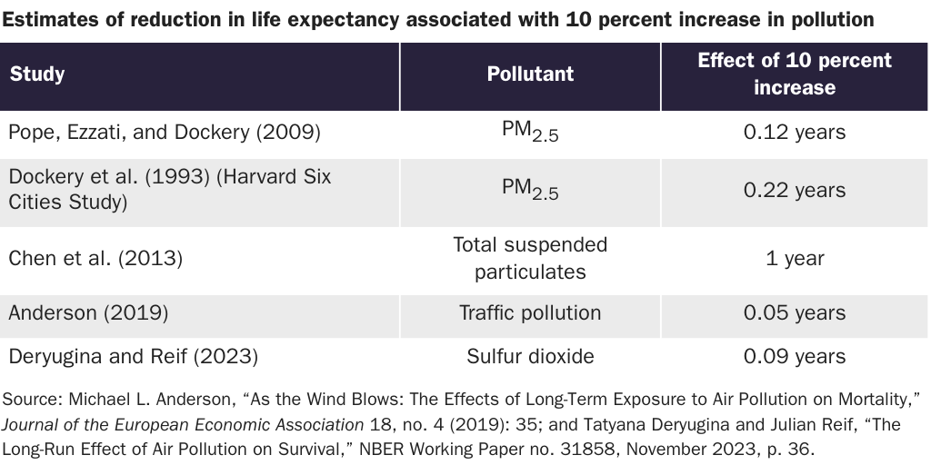
Thus, with the exception of Chen’s results, which are based on observations of much higher levels of pollution, the findings of quasi-experimental studies in the economic literature seem to be lower than the effects found by epidemiologists.
Regulating PM2.5: Calculating Costs and Benefits amid Scientific Uncertainty
Despite what we believe to be considerable uncertainty with estimates of the mortality effects of chronic PM2.5 exposure, the EPA has largely treated the matter as settled. While the ways in which the EPA sets and enforces standards has faced a good deal of criticism, little has changed since PM2.5 was first regulated in 1997. In fact, the processes are highly predictable.
Under the NAAQS process, the PM2.5 standards are reassessed every five years. When Republicans are in office, regulators determine that the most recent science does not support a lowering of the acceptable level of particulate matter, and so the status quo stands. When Democrats are in office, regulators determine that the science—sometimes the exact same research—is sufficient to justify tightening the standard. The potential benefits of a proposed change to the permissible level of PM2.5, as well as a few alternative changes, are assessed. While the benefits of the lowest proposed level are always the largest, the standard has always been set at a level that is slightly below the average level of exposure evaluated in the scientific studies used to justify the health benefits.
In 1997, the Bill Clinton EPA first began regulating PM2.5, setting the annual average standard at 15 μg/m³, about 1 μg/m³ below the mean of short- and long-term studies used to justify regulation of PM2.5.91 Under the George W. Bush administration, in 2006 the EPA elected to maintain the annual standard at 15 μg/m³, citing scientific uncertainty in the health effects of PM2.5 levels below those seen in the available evidence (the Bush EPA did lower the 24-hour standard from 65 μg/m³ to 35 μg/m³ based on available studies on the short-term health effects of particulate matter). In 2013, the Barack Obama administration lowered the standard to 12 μg/m³, again slightly lower than the mean concentration in the most recent long-term epidemiological studies.
In 2020, under the first Donald Trump administration, the EPA determined that the scientific evidence did not justify lowering the standard.92 Under President Joe Biden, the EPA reconsidered the 2020 decision and began the process to lower the standard, finalizing a rule that lowered the standard to 9 μg/m³ in February 2024.93
While the NAAQS does not allow for the consideration of costs, federal agencies are required to conduct a cost-benefit analysis for any “economically significant” regulation. Thus, the EPA conducts a regulatory impact analysis (RIA) of changing the PM2.5 standards, even though the findings are technically not going to have an effect on the ultimate decisionmaking process. A close reading of the RIA’s findings, and the assumptions involved, illustrate the many uncertainties of determining the costs and benefits of major regulations, as well as how federal agencies obscure these uncertainties.
The RIA for lowering the annual average standard for PM2.5 to 9 μg/m³ assesses the health benefits and control costs of the change and alternatives of 10 or 8 μg/m³, along with lowering the 24-hour standard from 35 to 30 μg/m³. It finds that the benefits of reducing PM to any level dwarf the estimated costs. Both avoided mortality and morbidity are considered, but the majority of benefits (over 98 percent) stem from avoided deaths.94 The mortality estimates are based on two sources. One is the 2020 paper by Wu, which estimates the mortality effects among the elderly population with a hazard ratio of 1.066 per 10 μg/m³ increase in PM2.5 exposure. The other is a 2019 study by C. Arden Pope III and colleagues that uses traditional methods to estimate a hazard ratio of 1.12 among the entire adult population.95 Depending on which estimate of avoided mortality is used and the discount rate, the health benefits of changing the standard to 9 μg/m³ are estimated to range from $20 to $46 billion per year (in 2017 dollars).
To estimate costs, the EPA determines which counties will need to reduce PM2.5 levels and identifies “illustrative” control strategies. Ultimately, the control strategies will be determined by states and counties, not the EPA. According to the EPA estimates, the costs of the identified control strategies would be about $594 million per year, and the benefits of the new standard are about 70 to 165 times larger than the costs.
Of course, the RIA, like any ex ante analysis of costs and benefits, requires assumptions to be made and must incorporate some level of uncertainty. The EPA acknowledges some sources of ambiguity. Estimates of future PM2.5 levels and the costs of control strategies are ultimately guesses based on current trends and available technologies. The benefits must incorporate the statistical uncertainties of the assumed health effects and economic valuation of deaths.
The EPA does not appropriately confront all forms of uncertainty when determining and evaluating NAAQS. Economists Anne E. Smith and Will Gans note that, while the EPA may appropriately incorporate reported statistical uncertainties, there are additional ambiguities that are omitted.96 These include questions about whether the damages of particulate matter are attenuated at lower concentrations and whether distinct components of PM2.5 have different levels of toxicity.
Furthermore, the EPA makes assumptions about the ability of states and counties to comply with the standards. Whenever the NAAQS is changed there are counties that fail to comply with the lower standard, including a group of counties with a sizeable population that has been in “nonattainment” with the PM2.5 standards since the outset. The EPA falls short of assuming that all counties will manage to achieve the new PM2.5. But its analysis does assume PM2.5 reductions, which should not be taken as given.
Altogether, these uncertainties, along with the continuing debate over the health effects of PM2.5, suggest a less clear cost-benefit ratio than the EPA implies.
The Concentration-Response Relationship
The NAAQS and RIA rely on the assumption that the relationship between mortality and PM2.5 is linear and exists even at low levels of PM2.5. Levels of particulate matter in the United States are already lower than they were during the periods in which the epidemiological research used to estimate health benefits was conducted. Thus, even ignoring any potential flaws in those studies, justification of lowering the standards requires us to suppose that the observed health benefits will continue at levels lower than have been observed.
To support its estimated health benefits, the EPA assumes that the relationship between the concentration of PM2.5 that people are exposed to and the response (in this case mortality) is linear and has no threshold. As demonstrated in Figure 1, this type of concentration-response relationship (C‑R relationship) has a constant slope from high levels of PM2.5 exposure down to zero. In other words, the health benefits used assume that a 10 μg/m³ decrease in PM2.5 concentration has the same effect whether the change is from 50 μg/m³ to 40 μg/m³ or from 15 μg/m³ to 5 μg/m³. Moreover, the EPA assumes that there is no threshold below which particulate matter ceases to affect human mortality. The EPA contends that results of studies using a variety of statistical methods support the theory of a linear, no-threshold C‑R function for PM2.5. 97
![Copy: Figure 1 [print]: PM C-R Functions](https://infogram-thumbs-1024.s3-eu-west-1.amazonaws.com/f66639e0-11de-4ba6-b896-f3fe68c2efaf.jpg)
This assumption has long been criticized.98 It is possible that the threshold is lower than the levels of exposure in observational studies to date and therefore has so far been difficult to detect. This would imply that, as PM2.5 concentrations continue to decline, we will at some point begin to detect a threshold. More importantly, though, measurement error (the difference between “observed” and “true” PM2.5 exposure) makes it difficult to detect a threshold, even if that threshold is already well within the range of observed concentrations. In a 2022 analysis, Garrett Glasgow, Bharat Ramkrishnan, and Anne E. Smith used simulations to demonstrate how measurement error can obscure a threshold.99
The existence or nonexistence of a threshold is crucial to evaluating the benefits of lowering PM2.5 standards. A linear, no-threshold C‑R relationship, as illustrated in Figure 1, would mean continued benefits as PM2.5 levels are further reduced. If the threshold function represents the true C‑R relationship, and the threshold is somewhere within the current range of PM2.5 concentrations in the United States, then the real benefits of lowering the standard are less than the EPA estimates. If PM2.5 levels are already below the threshold, the actual benefits of reducing the standard would be zero.
Epidemiologists have also recently asked whether the C‑R relationship is, in fact, “supralinear”—that is, it has a steeper slope at lower concentrations than at higher concentrations. Extrapolation of the estimated mortality effects of PM2.5 from developed Western countries with low concentrations (e.g., annual averages of 5 to 30 μg/m³), where the health effects were observed, meant implausibly high levels of mortality in countries such as China and India that have much higher levels of particulate matter (annual averages can be more than 100 μg/m³).100
In 2015, for example, average annual PM2.5 level in New York City ranged from 7.2 μg/m³ to 12.3 μg/m³ by neighborhood.101 The average annual concentration in Delhi was 112.1 μg/m³.102 Linear extrapolation of the health benefits used by the EPA implies that a 100 μg/m³ difference in PM2.5 means the all-cause mortality rate would be nearly 90 percent higher among the elderly population (i.e., aged 65 and over) and more than 200 percent higher among all adults.103 In 2015, the crude death rate for all ages in New York City was 6.3 per 1,000 people compared to 6.8 per 1,000 in Delhi—an 8 percent difference.104 If the effects of PM2.5 exposure are assumed to be linear, then it is surprising that the mortality impacts are not more immediately obvious.
Faced with the disconnect between observed mortality and PM2.5 exposure rates, epidemiologists have argued that the marginal effects of exposure at lower concentrations may actually be larger, as demonstrated by the supralinear C‑R function in Figure 1: The health effects are large at relatively low levels of exposure but plateau at higher levels.105
Whether the C‑R function is supralinear is important for estimates of the benefits of reducing air pollution. If this relationship is correct, it implies that there are still substantial benefits to be achieved in countries such as the United States, which have already low concentrations of PM2.5.106 The supralinearity of the C‑R function has been supported by some recent research. For example, Wu’s 2020 paper assesses overall elderly mortality caused by PM2.5 and the mortality caused only among the population that was consistently exposed to PM2.5 less than 12 μg/m³.107 They find that the relative risk of the low-exposure group is higher than that of the full population. Additional research has focused on populations in Canada and Europe exposed to low-levels of particulate matter and found evidence of supralinearity.108
However, the credibility of a supralinear C‑R relationship has been questioned.109 Additional research by Glasgow and colleagues again uses simulations to illustrate conditions in which statistical analyses may observe a false supralinear C‑R function.110 Their analysis finds that differences in the composition of ambient PM2.5, the presence of unmeasured confounding variables correlated with PM2.5, or certain types of measurement error could all lead to the incorrect finding of a supralinear relationship.
Without conclusive evidence of the form of the C‑R relationship, the EPA has assumed that it is linear. This may underestimate (in the case of a true supralinear relationship) or overestimate (if there is a threshold) the benefits of further PM2.5 regulation. Given the potential for current statistical methods to falsely identify a supralinear function and the methods’ difficulty in detecting a threshold, questions about the mortality effects of PM2.5 will likely persist. The EPA’s decision to ignore these questions means it understates the true uncertainty of the estimated benefits of PM2.5 reductions.
Differences in the Constituents and Sources of PM2.5
Unlike other air pollutants regulated by the CAA, particulate matter does not refer to a specific chemical but instead refers to a variety of components with different attributes. Evidence suggests that different components of PM2.5 have differing levels of toxicity, and emissions from different types of sources are transported different relative distances. Uncertainty about which sources and types of particulates have higher or lower levels of toxicity, and the local nature of the way in which the EPA currently regulates particulate matter, implies the existence of substantial inefficiencies in PM2.5 regulation.
PM2.5 is a regulatory category based on particle size (particles and droplets with a diameter of 2.5 micrometers or less) rather than on chemical or physical composition or source. The range of constituents that fit within this classification runs a wide gamut of organic and inorganic substances from both human (anthropogenic) and natural (biogenic) sources. It comprises emissions from fuel combustion, such as from coal-burning power plants; transportation, including from on-road vehicles such as cars and trucks and off-road vehicles such as trains and airplanes; industrial activities; dust from agriculture, construction, and paved and unpaved roads; and from natural sources such as wildfires, dust storms, and sea salt.
Particles that are directly emitted by a source into the air are considered primary PM2.5. Secondary PM2.5 are particulates formed by chemical reactions between gases in the atmosphere.111 Two of the most important secondary particulates are sulfates and nitrates. Historically, the largest source of the precursor gases that create sulfates has been power plants, especially coal-burning power plants. The largest source of the precursors of nitrates is transportation, including both on- and off-road vehicles.112
Composition of particulate matter differs by location and has changed over time. Particulate matter from traffic and soil is found across the United States, while PM2.5 from specific industries (e.g., metals processing) is found in more industrialized areas.113 Historically, sulfates made up a large proportion of particulate matter in the eastern United States, where coal combustion was prominent. In the western United States, on the other hand, nitrates have made up a larger relative portion.114 However, a large part of the decrease in PM2.5 over the past couple of decades is the decline in both sulfates and nitrates, driven by reductions in emissions from power plants (especially diminishing sulfates from coal-burning power plants) and mobile sources (on- and off-road vehicles).115
Grouping all substances of a certain size into one regulatory category assumes that different chemicals and sources have the same levels of toxicity or require the same national-level intervention. If there are differences in how dangerous the different components of particulate matter are, or if there are ways in which PM2.5 can be dealt with more locally, it is possible that the current regulations are overestimating the benefits or regulating PM2.5 inefficiently.
Toxicity
To date, toxicological and epidemiological research suggests that different components of particulate matter cause differing levels of health damage, but attempts to resolve which constituents can be considered more or less dangerous have been inconclusive.116 Confounding factors and correlations between different components of PM2.5 make it difficult to draw definitive conclusions. The EPA has so far determined that there “is not sufficient evidence to differentiate the components or sources more closely related to health outcomes when compared with PM2.5 mass.”117
The evidence does seem to support the notion that different components and sources do have different effects. For example, an evaluation of the toxicity of various sources found that diesel and gasoline exhaust particles, biomass burning, coal combustion, and paved road dust were the most toxic.118 Meanwhile, the analysis found that natural dust, while still demonstrating some toxicity, was less harmful.
An important distinction is between road dust and natural dust, as well as between dust from paved versus unpaved roads. Road dust from paved roads consists largely of particles from brake, tire, and road wear.119 This dust can be resuspended in the air by the movement of vehicles on the road. Natural dust largely consists of crustal materials (i.e., soil) and is often resuspended by wind. Road dust from unpaved roads is also mostly soil.120 More dust is emitted from vehicles traveling over unpaved than paved roads.121 However, it likely has health effects similar to natural dust.
Epidemiological evidence on the long-term health effects of components of particulate matter are subject to the same concerns of confounding, measurement error, and migration effects. And research that attempts to assign different components of PM2.5 to particular sources are additionally subject to any uncertainties or bias that arises from the apportionment process.
However, analyses of the long-term mortality associated with different components and sources have generally found larger effects of particulate matter from fossil fuel and biomass combustion (which are the sources of substances including black carbon, organic matter, sulfates, and nitrates) and smaller effects for soil.122 A review of studies on the short-term health effects of particulate matter components found that emissions from traffic, coal-burning power plants, and diesel exhaust were consistently associated with a variety of cardiovascular and respiratory health outcomes, including mortality, while wood smoke had mixed results and soil was consistently found not to have a statistically significant effect.123
A study in the United States found that PM2.5 exposure from coal combustion and diesel exhaust were associated with ischemic heart disease mortality, while biomass burning and wind-blown soil had no effect.124 Similarly, research on cardiovascular mortality in China found that particulate matter constituents from fossil fuel combustion had higher relative risks while soil dust had no risk.125
An initiative by the Health Effects Institute combined epidemiological and toxicological attempts to differentiate between the health effects of differing components.126 It found that PM2.5 from coal and oil combustion, and to a lesser extent traffic, were associated with adverse health outcomes. However, the institute determined that it could not rule out adverse effects of other components or sources.
The research seems to indicate that coal combustion and traffic emissions are found to consistently have adverse health effects. But in the EPA’s assessment of the regulatory impact of changing the NAAQS it does not consider any control measures that would limit emissions from coal-burning power plants or vehicle tailpipes. This is in part because the agency’s baseline projections for future PM2.5 include substantial declines in emissions from these sources, partly stemming from existing regulations.127 If the health effects of total PM2.5 are disproportionately caused by coal and automobile emissions, and the RIA does not predict that changing the NAAQS will cause any reduction in these emissions, then the total benefits of the RIA are overestimated.
On the flip side, one of the most substantial control strategies identified by the EPA in the RIA is the paving of unpaved roads and unpaved road shoulders. It accounts for roughly 16 percent of the reduction in PM2.5 and 64 percent of the estimated control costs.128 To the extent that existing epidemiology is correct that soil is generally less harmful than other PM constituents, and that dust from unpaved roads and road shoulders is largely soil, then the benefits are again overestimated.
Overall, regulating based on a physical characteristic (particle size) that does not match up exactly with the toxicity of the particles is inefficient. This is especially true if the relative toxicity of emissions from different sources does not align with the relative control costs. If the most toxic source also happens to be the easiest to directly address, as may have happened with coal-burning power plants, then regulating based on total PM2.5 mass may be effective. However, any health benefits are coincidental. If the easiest control strategies address the least-harmful or nonharmful sources, as may be the case with paving unpaved roads, then the targeted PM2.5 reductions may be achieved, but without the coincidental health benefits. As long as regulation of PM2.5 is based on total mass, instead of identifying and addressing the most harmful sources, there will be uncertainty in the effectiveness of the government intervention.129
Transport
The location and source of PM2.5 emissions significantly affect health outcomes. The distance PM2.5 is transported and the overlap of emissions with the population determine the amount of pollution that is inhaled and, ultimately, the health effects experienced. PM2.5 can be a regional problem, with sizable damages occurring in areas outside of where the pollution is emitted. However, the RIA and the NAAQS deal with PM2.5 on a county level. While this suggests that PM2.5 pollution is becoming a more localized issue, the EPA is still ignoring within-county variation in emissions that may affect the effectiveness of the control strategies.
Under certain conditions and from specific sources, PM2.5 can travel long distances. For example, wildfires in the western United States can affect air quality in the east, and dust storms in the Sahara can transport particulates to the southern United States.130 A small amount of the particulate matter in the United States is emitted by industrial sources in China.131
Emissions from elevated smokestacks can travel hundreds of miles, whereas ground-level sources disperse within shorter distances.132 Because sulfates and nitrates form in the atmosphere from chemical reactions of precursor gases such as sulfur dioxide and nitrogen oxides, they can have much longer ranges. Primary PM2.5 has a shorter range. For example, mobile sources cause PM2.5 concentrations to sharply increase near roads, but these spikes dissipate within a few hundred meters.133
The effect of these varying transport distances is that there is a relatively uniform level of background PM2.5 across a region, with higher concentrations in urban areas that are close to PM2.5 sources.134 The anthropogenic share of the background level is largely sulfates and nitrates—secondary PM2.5 formed from gases that were likely emitted by relatively distant sources and dispersed over a wide region.135
In rural areas with fewer local sources of pollution, PM2.5 is mostly the background concentration. For example, research found that PM2.5 in the rural midwestern United States is mainly sulfates and nitrates (i.e., secondary PM2.5) and dust with some particulates from local sources such as vehicle emissions.136
As illustrated by Figure 2, cities and more densely populated areas have higher concentrations of PM2.5 compared to rural regions, an increase known as the “urban increment.” This increment, on top of background PM2.5, is created by primary emissions from local sources, which are more concentrated in urban areas. The range of primary PM2.5 is typically much smaller than secondary PM2.5, meaning that differences in PM2.5 can be highly localized, with research showing that there are substantial intra-urban variations down to the one-kilometer (km) level (about 0.62 miles).137
![Copy: Figure 2 [print]: Kemp_Van Doren_Air Quality Regulation](https://infogram-thumbs-1024.s3-eu-west-1.amazonaws.com/7fac2f85-c0bb-49cf-b66d-d6c951d64ed8.jpg)
The health damage caused by a source depends on how the spatial extent of its pollution overlaps with the population.138 Although elevated emissions travel farther, ground-level local emissions may be more damaging because they are more likely to be inhaled by people.139
The RIA does not explicitly consider transport of particulate matter or the spatial extent of emissions when identifying potential control strategies. It focuses on the county level and on methods to reduce primary PM2.5. The EPA argues that its “approach is consistent with the exceedances generally being driven by the urban PM2.5 increment, the relatively high responsiveness of PM2.5 concentrations to primary PM2.5 emission reductions, and the reductions in regional PM2.5 concentrations from the large SO2 [sulfur dioxide] and NOx [nitrogen oxides] emission reductions in recent decades and in the 2032 projection.”140
However, this ignores the fact that primary PM2.5 emissions can be highly localized and it assumes that reductions in emissions will be felt uniformly across a county. In actuality, the health benefits will be only realized as far as the control strategies address emission sources that the county’s population is actually exposed to. Because the spatial extent of emissions sources is ignored, as in the questions of source toxicity, any realized benefits are coincidental.
In urban areas, for example, much of the spatial difference in PM2.5 is caused by emissions from mobile sources and commercial cooking.141 A sizable portion (about 24 percent) of the reduction in PM2.5 estimated in the RIA stems from envisioned controls on commercial cooking emissions.142 Although restaurant emissions have a small spatial extent (several hundred meters), evidence suggests that restaurant density is correlated with population density.143 As long as emissions from commercial cooking are assumed to be as toxic as other emissions, reducing cooking emissions may have sizeable health benefits.
On the other hand, paving dirt roads may be effective at reducing the average ambient PM2.5 level of a county, but if dust emitted from dirt roads has a relatively small range, and dirt roads are expected to be in areas with lower population density, then the actual reduction in particulates inhaled by people, and thus the estimated health benefits, may be overstated.
Excluding the variation in PM2.5 transport and the spatial impact of sources reduces the efficiency of PM2.5 regulation as well as the estimated benefits.
Dubious Cost and Benefit Assumptions
The accuracy of the projected benefits and costs in the RIA relies heavily on assumptions about counties’ abilities to control PM2.5 emissions. The RIA acknowledges that some counties have historically been unable to achieve the NAAQS and are classified as nonattainment areas. However, the RIA may overestimate these counties’ capacity to partially comply with the new standard, while also failing to account for the costs associated with nonattainment.
The EPA designates nonattainment status based on a county’s design value (DV), a three-year average of annual PM2.5 concentrations.144 The RIA forecasts county annual DVs to 2032.145 In counties with projected levels above 12 μg/m³—those that are still in nonattainment with the 2012 NAAQS—the EPA identifies control strategies to reduce PM2.5 concentrations to 12 μg/m³. The benefits and costs of these reductions are excluded from the RIA’s final estimates. After establishing a 12 μg/m³ baseline, the EPA then outlines which counties are projected to have PM2.5 levels above the new 9 μg/m³ standard and assesses available control strategies.
According to the RIA, only a small number of counties will be affected by the lower PM2.5 standard.146 Out of 3,108 counties in the contiguous United States, only 52 are projected to exceed 9 μg/m³. In the northeast and southeast, where counties tend to be smaller, the EPA also includes emissions reductions in 19 neighboring counties to help improve air quality in an adjacent core county. Figure 3 displays the small number of counties affected by the new standard.
![Copy: Figure 3 [print]: Kemp_Van Doren_Air Quality Regulation PM RIA county map](https://infogram-thumbs-1024.s3-eu-west-1.amazonaws.com/e401ade3-ff2f-46aa-a13f-6f714603995c.jpg)
While the EPA acknowledges that some counties may struggle to meet the new 9 μg/m³ limit, it projects that 25 of the 52 core counties will require reductions beyond the available control strategies. This includes Riverside and Plumas counties in California, where the EPA is unable to identify any strategies for reducing emissions below 12 μg/m³.
In a sense, then, the RIA is incomplete. According to the letter of the CAA, these 25 counties would still be obligated to achieve reductions to meet the new standard, implying additional costs and benefits not accounted for in the RIA. The costs of achieving these reductions are likely to be high, as most easily identifiable control strategies have already been utilized.
However, the EPA’s prediction that many counties will be noncompliant reflects the historical reality. As of August 2024, 15 counties were wholly or partially in nonattainment with the 2012 NAAQS, corresponding to a population of nearly 21 million people.147 Notably, 13 of these counties have been designated nonattainment areas since the first PM2.5 standard was established in 1997. This pattern has been called “institutionalized nonattainment.”148
Although it is appropriate to project that some counties remain in nonattainment, the EPA makes questionable assumptions about PM2.5 reductions in areas with a history of nonattainment. The RIA additionally only includes the costs of control strategies, ignoring costs associated with nonattainment status.
Costs of Nonattainment Status
Polluting industries in nonattainment areas face strict regulations that increase the cost of building or expanding facilities. Most importantly, major new emissions sources and major modifications to existing sources are required to meet the most stringent emissions limitation under the CAA’s lowest achievable emissions rate without any consideration of the costs involved.149 Furthermore, any new emissions must be offset by equivalent or greater emissions reductions elsewhere in the county.
These regulations can impose substantial costs on industries. For example, economist Randy Becker studies air pollution abatement costs for manufacturing plants from 1979 to 1987.150 He finds that, on average, plants in areas in nonattainment with any CAA criteria pollutant experienced abatement costs hundreds of thousands of dollars more than plants in attainment areas (in 1987 dollars). In an analysis of ozone nonattainment between 1972 and 1992, Becker and Vernon Henderson find that the average total costs of plants in nonattainment areas were roughly 4 to 18 percent higher than in attainment areas, depending on the industry and plant age.151
Economic research has also determined that nonattainment reduces both output and employment, and it ultimately causes industries to change behavior in economically inefficient ways. In a separate study, Becker and Henderson analyze plant data from 1963 to 1992 and find that nonattainment with the ozone NAAQS led polluting industries to relocate to less polluted places and to open smaller plants to avoid the more stringent regulations.152 Since these shifts were toward less-productive areas and required industries to operate at less-efficient scales, they created welfare losses that, at least partly, offset any benefit of the air quality regulation.
Similarly, Michael Greenstone finds that, in the first 15 years the CAA was in effect (1972 to 1987), counties in nonattainment with four criteria air pollutants (carbon monoxide, ozone, sulfur dioxide, and total suspended particulates) lost about 590,000 jobs, $37 billion in capital stock, and $75 billion in output (both in 1987 dollars).153 He mentions that, from a national level perspective, these are likely overestimates because some portion of industrial activity in nonattainment counties will have shifted to attainment counties.154 But the costs of these adjustments can be substantial and persistent. What matters from a nonattainment county’s perspective, though, is the absolute loss in jobs and output.
Additional research by Greenstone, John A. List, and Chad Syverson estimates that, from 1972 to 1993, total factor productivity decreased by 4.8 percent in counties in nonattainment with the same four criteria pollutants, translating to an annual loss of $21 billion (in 2010 dollars).155 Looking at the labor effects of the 1990 CAA amendments, W. Reed Walker finds that workers at newly regulated plants saw their earnings decrease by 20 percent after their counties were designated as nonattainment, amounting to an aggregate loss of $5.4 billion (in 1990 dollars).156
While these studies focus on pollutants other than PM2.5, the economic effects of nonattainment are likely to apply to PM2.5 as well. The stringent regulations on polluting industries can lead to higher costs, shifts to less-efficient locations or plant sizes, and losses for both industries and workers. The RIA fails to account for these economic costs.
Recent Trends in PM2.5 Concentration in Permanent Nonattainment Counties
Although the EPA recognizes that some counties may remain in nonattainment, with the exception of Riverside and Plumas counties, California, it still assumes reductions in PM2.5 in 50 of the 52 core counties. Is this assumption consistent with recent trends?
Since the 2011–2013 DVs—the last period before nonattainment with the 2012 NAAQS was designated—PM2.5 levels in many core counties have remained flat and, in some cases, have increased. As shown in Figure 4, concentrations in the 13 permanent nonattainment counties did decrease, on average, after the 1997 NAAQS but have generally remained level in the past decade. Between the 2001–2003 and 2011–2013 periods, in those 13 counties the DV, on average, decreased by roughly 0.58 μg/m³ per year. However, from 2012–2014 to 2021–2023 the average reduction was only about 0.17 μg/m³ per year.157
![Copy: Figure 4 [print]: Kemp_Van Doren_Air Quality Regulation PM recent DVs](https://infogram-thumbs-1024.s3-eu-west-1.amazonaws.com/17c39f70-cad2-4546-bc3f-ba6241294692.jpg)
The difference is partly the result of increases in some counties. For example, in Los Angeles County, where a substantial portion of the estimated benefits of the new NAAQS are concentrated, for 2011–2013 the DV was 12.5 μg/m³ while in 2020–2022 it was 13.4 μg/m³. Los Angeles County’s 2021–2023 DV of 12.2 μg/m³ marks the first time since the 2012 NAAQS that its PM2.5 concentration dipped below the 2011–2013 level.
What ultimately matters in the RIA’s calculation of benefits is the change in PM2.5 level. If the PM2.5 DV increases, none of the estimated benefits will occur. But a smaller than projected decrease in PM2.5 concentration also means that the benefits will be less than estimated. This is again particularly important for Los Angeles County. The RIA projects that the county will have a decrease of about 1.3 μg/m³.158 However, the recent decline to 12.2 μg/m³ is only 0.3 μg/m³ less than the DV in 2011–2013, meaning that it has taken Los Angeles County a decade to lower its DV by less than a quarter of the future reduction projected by the RIA.
This history suggests, since the EPA ignores the costs of nonattainment and questions about key counties’ abilities to control PM2.5 emissions, that the true costs are higher and the benefits are lower than the RIA’s estimates.
Local Costs and Benefits
According to the RIA, the annual benefits of avoided mortality created by the recent NAAQS change are $22 to $46 billion per year for Wu’s and Pope’s health impacts, respectively (in 2017 dollars and at a 3 percent discount rate). The annual costs are about $594 million.
However, the RIA and NAAQS focus on reducing PM2.5 at the local level, and the identified control strategies explicitly forgo any attempt to lower emissions from regional (e.g., power plants) or mobile sources. Thus, it is important to consider whether the regulation passes a cost-benefit test at the county level.
That information has not been publicly released. While the EPA has privately shared data on emissions reductions and costs by county, the county-level breakdown of benefits is not available. Using the data on emissions reductions and roughly following the methods outlined in the RIA, we estimate the annual number of deaths avoided and the monetized benefits in each county with projected emissions reductions (50 core counties, excluding Riverside and Plumas Counties, California) using both Wu’s and Pope’s health effects. Because the 19 neighboring counties identified by the EPA only reduce emissions to help lower ambient PM2.5 in an adjacent county, we combine the benefits and costs of neighboring counties into the adjacent core counties. Our full methodology and detailed breakdown of the avoided deaths, benefits, and costs are outlined in the appendix.
As summarized in Table 3, our overall results are similar to the results of the RIA. The small discrepancy likely stems from simplifications of our analysis. Our overall results are higher than those in the RIA, suggesting that we may also overestimate the benefits at the county level.
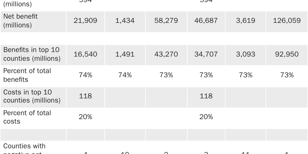
Like the RIA, we report the point estimates, along with the 2.5 and 97.5 percentile estimates. These represent the 95 percent confidence interval of the benefits as derived from the statistical uncertainties of the mortality effects and of the valuation of avoided mortality.
Separating the effects by county immediately highlights that the benefits of regulation are highly concentrated, whereas the costs are largely dispersed. The top 10 counties (one-fifth of the 50 included counties) in terms of avoided mortality receive more than 70 percent of the total benefits.159 These same 10 counties only pay 20 percent of the total costs. Los Angeles County alone receives 25 percent of the total benefits, while only bearing 2 percent of the costs.
The benefits are not uniform across counties because of population variation. The top 10 counties contain slightly more than half of the total population of the 50 counties. Thus, the same decrease in PM2.5 in those counties will be estimated to result in a larger number of avoided deaths. And the control costs in those counties are also spread across a larger population. The per capita annual cost in the 10 counties is $5.33.
The reverse is true of the bottom 40 counties. Having a lower population means that the estimated benefit of the same reduction in PM2.5 will be lower, while the costs are borne by a smaller number of residents. The average per capita cost in the bottom 40 counties is $95.64. On the extreme end is Lincoln County, Montana, where $27 million in control costs spread across a resident population of about 22,000 would imply a per capita cost of approximately $1,230 each year.
These results suggest that the balance between benefits and costs at the county level varies widely. In fact, three or four counties have negative net benefits, according to the point estimates of avoided mortality.
If we restrict our analysis to the lowest benefit estimates within the 95 percent confidence interval, the number of counties with negative net benefits increases. At the 2.5 percentile level, 11 to 19 counties (roughly one- to two-fifths) have net negative benefits. These counties account for roughly 20 to 60 percent of the total costs. The benefits estimated for all counties at the 2.5 percentile are 3.4 to 7 times the costs, while the benefits in the bottom 40 counties are only 1.3 to 2.4 times the costs. (In the top 10 counties, the 2.5 percentile benefit-to-cost ratio is still 13 to 26.)
These negative conclusions accept the findings of Wu and Pope and the RIA’s existing level of uncertainty without qualification. If the criticisms we have discussed in this paper are valid, then the benefits are even lower.
Comparing benefits and costs at a local level makes it difficult to justify the regulation. For example, residents of Shoshone County, Idaho, where the majority of annual PM2.5 emissions is dust rather than vehicle emissions, and where the costs of control will more than likely exceed the estimated benefits, might have difficulty comprehending why they may be forced to pay more than $900 per year to pave rural dirt roads for little local benefit.160
Policy Recommendations
In an ideal world, science would offer definitive answers to questions about the effect of exposure to PM2.5 on health. But science seems unlikely to provide these definitive answers. And even if it could, policy can only be informed by, rather than based on, science. Peter Van Doren explains in his 2020 essay on the role of science in COVID-19 policy:
At its best, science explains relationships between cause and effect: no more and no less. No normative conclusions about individual or collective decisions follow directly from science. Instead costs, benefits, and other values properly enter both individual and collective decisions.161
In the case of ambient air quality standards, even if science could conclusively tell us how PM2.5 affects mortality, it would still not provide a clear recommendation of what the acceptable level of pollution should be. The NAAQS should be reformed to better account for uncertainty, other normative factors, and creating opportunities for more localized decisionmaking.
Acknowledging Uncertainty
Scientific uncertainty is a central challenge in regulating PM2.5. While quantitative analyses of PM2.5 benefits include 95 percent confidence intervals to account for statistical uncertainty, they overlook deeper uncertainties, such as incomplete knowledge about key processes and relationships.
A 2002 National Research Council report criticized the EPA for failing to address these uncertainties. It described the many potential sources of uncertainty that are ignored:
Areas of uncertainty include air-quality modeling, population demographics and heterogeneity, intersubject variability, health and exposure baselines, compliance with control measures, effectiveness of controls in reducing pollutant emissions, validity and precision of concentration-response functions and use of alternative models (linear, nonlinear), estimation of these functions as relative effects (relative risks) or absolute effects (risk differences), relative toxicity of mixture components, and applicability of these functions to target populations of regulatory concern. These uncertainties are rooted in incomplete scientific knowledge. When benefits are estimated for future target populations, the cumulative magnitude of the uncertainties can be formidable. Many of them can be reduced by further research, but on the whole, they are likely to remain high.162
Economists Art Fraas and Randall Lutter revisited this issue in 2013 and found that little progress had been made.163 They show that different assumptions about mortality risk, concentration-response relationships, and PM2.5 toxicity dramatically alter estimates of benefits.
For the past decade, economist Anne Smith has explored various methods of including the full scope of uncertainty within the NAAQS process. For example, in a 2014 study she and Will Gans propose improvements to the Environmental Benefits Mapping and Analysis Program (BenMAP), the EPA’s open-source software for estimating the public health risks of air pollution, to better assess sensitivity to uncertainty.164 In a 2018 paper, Smith argues for the inclusion of subjective uncertainty in the NAAQS assessment of risk.165 She outlines an expert elicitation process that, as long as methods to limit cognitive bias and properly weight expert judgments could be implemented, might help inform the risk assumptions and results of the NAAQS process.166 (From 2003 to 2006, the EPA did use expert elicitation on the C‑R function to inform RIAs, but not the NAAQS.)
Incorporating Costs
It has long been recognized that ambient air quality standards are ill-suited to regulation of pollutants such as PM2.5. In 1977, chemical engineer Noel de Nevers outlined the philosophies underlying air pollution control frameworks. He notes that “the air quality standards philosophy is based on the assumption that the true situation for most major air pollutants is the ‘threshold value’ situation,” [emphasis in original] and that, if the assumption is true, then it is, in theory, possible to implement a standard that means there is zero air pollution damage.167 However, de Nevers also acknowledges that if the threshold assumption is proven false—or, as we contend, whether there is no threshold or the threshold simply cannot be detected—then:
It will be equally clear that the ambient air quality standard or zero-damage philosophy is without intellectual foundation. If that is the case, we will still be able to use ambient air quality standards if we wish; but we will have to choose the values on some philosophical basis entirely different from that used to date.168
As time has progressed, de Nevers’s assessment of the ambient air quality standards has proven increasingly relevant. Whether it is because there is no threshold, or because we have been unable to detect one, science has not offered a level of PM2.5 exposure that results in “zero damage.” Nevertheless, the Supreme Court’s ruling in Whitman v. American Trucking Associations, Inc. restricts the EPA to only consider the concentration at which there is the lowest level of risk. This leads to what legal scholars Michael Livermore and Richard Revesz describe as the “stopping-point problem”:
The complete elimination of health risks for these pollutants could be accomplished only by banning all emissions. Such stringent standards would lead to widespread social dislocation and even strongly pro-environmental commentators regard them as undesirable. But when costs cannot be considered, it is difficult to justify any stopping point other than zero.… Under the standard reading of American Trucking, EPA faces the choice either to impose crushing social costs—which would be politically reckless—or to determine an acceptable non-zero level of risk without reference to any social goal other than health, which would be an incoherent task.169
In practice, the EPA does implicitly consider costs by not setting the NAAQS at zero, even though it cites science as the sole basis for its decisions. This lack of transparency obscures the real tradeoffs and stifles open discussion about the costs of regulation.170 Addressing this requires legislative reform; the current legal framework prevents the EPA from fully incorporating economic considerations into its decisions.171
Reorienting Federal, State, and Local Involvement
As federal regulation of air pollution was being discussed in the 1960s, a key question was whether standards should be established at a national level or whether they should be determined by state or local governments. The 1970 CAA amendments ultimately created both national-level emissions and ambient air quality standards. However, the uneven geographic distribution of the costs and benefits of further PM2.5 regulation, and the contrast between dusty rural counties in Idaho and urban counties in Southern California that are in permanent nonattainment, suggests that uniform national standards fail to account for local variations in meteorology, geography, urbanization, and industrialization.
National standards are often justified by the issue of interstate pollution. But research shows that this share has been declining.172 And the geographic scale of the problem for PM2.5 depends in large part on the constituents and sources.
For example, one study found that, in 2011, 41 percent of mortality related to PM2.5 was attributed to cross-state emissions. The share of cross-state deaths for sulfates and nitrates was higher (77 and 52 percent, respectively) compared to primary PM2.5 emissions (35 percent). The study also found that mortality caused by cross-state emissions declined from 2005 to 2011. Separate research found that half of the damages of PM2.5 occur within 32 km (around 20 miles) of the source.173 More than half of the damages of sulfur dioxide (the precursor of sulfate) occur more than 200 km (about 125 miles) from the source, whereas more than half of primary PM2.5 damages occur within less than 16 km (10 miles).
Although cross-state emissions are declining, interstate PM2.5 pollution will remain a policy issue because there are incentives (for both governments and firms) to locate polluters in places where emissions will be transported out of their jurisdiction. Both industrial sources and power plants strategically locate close to a downwind border.174
These concerns provide a reasonable justification for federal involvement in the regulation of interstate pollution. Ironically, this is an area where the EPA has proven to be the least effective. The Clean Air Act’s good-neighbor provision requires states to limit emissions that “contribute significantly to nonattainment” in another state.175 Historically, the EPA has been reluctant to use the provision or has faced substantial legal obstacles when it has tried to do so.176 Recently, the EPA has put in place regional strategies to tackle the interstate transport of ozone, including the Cross State Air Pollution Rule and the Good Neighbor Plan; however, the latter has been put on hold by the Supreme Court amid ongoing legal challenges.177
One of the reasons for these challenges may be the EPA’s reliance on adapting existing legal frameworks to address interstate pollution. If pollution from sources such as coal-burning power plants requires federal intervention, Congress should enact laws specifically tailored to address this issue. Instead, the EPA has tried to stretch the scope of existing legislation, often with questionable effectiveness and uncertain legal outcomes.
Research on regional air quality controls suggests that cap-and-trade schemes are generally more cost-effective than traditional command-and-control regulations. Cap-and-trade sets a cap on the total allowable emissions and issues tradable permits, allowing companies that reduce their emissions to sell excess permits to those that need them. This market-based approach enables emissions reductions to be achieved in a more economically efficient manner. While some US cap-and-trade programs, such as the sulfur dioxide program from the 1990 CAA amendments, have not always delivered the expected cost savings, they have typically outperformed traditional regulatory methods when they are properly designed.178
However, although interstate pollution may require federal intervention, this does not, in and of itself, justify continued use of a national-level ambient air quality standard. In fact, the NAAQS are not well suited to addressing interstate pollution and, in some ways, they incentivize it. As Revesz notes:
Federal ambient air quality standards are not well-targeted to address the problem of interstate externalities. They are overinclusive because they require a state to restrict pollution that has only in-state consequences. But they are also underinclusive because a state could meet the applicable ambient standards but nonetheless export a great deal of pollution to downwind states (through tall stacks or a location near the interstate border). In fact, a state might meet its ambient standards precisely because it exports a large proportion of its pollution.179
Furthermore, the EPA itself argues that, because of trends in the constituents and sources of PM2.5, efforts to further reduce PM2.5 will focus on controlling local sources. In the RIA for the recent PM2.5 NAAQS change it notes:
Conceptually, PM2.5 concentrations in urban areas can be viewed as the superposition of the urban increment and the contributions from regional and natural background sources. The decreases in anthropogenic SO2 and NOx [sulfate and nitrate] emissions in recent decades have reduced regional background concentrations and increased the relative importance of the urban increment. The projections of additional large reductions in SO2 and NOx emissions … further motivate the need for control of local primary PM2.5 sources to address the highest PM2.5 concentrations in urban areas.180
Thus, we propose eliminating the PM2.5 NAAQS and transferring responsibility for air quality regulation to state governments. The EPA could still offer guidance, research, and technical support, while continuing to regulate interstate and mobile sources of pollution. Considering the generally low PM2.5 concentrations in most of the United States and the local focus of future emissions controls, federal regulation of ambient PM2.5 is increasingly unnecessary.
In determining whether and how to further regulate PM2.5, state and local governments still face the same issues of determining how to incorporate the scientific evidence, including how to account for uncertainties created by our lack of knowledge. However, delegating the responsibility to state governments has several advantages.
First, federal control has increased administrative complexity and reduced accountability. In a 1996 proposal for reforming the EPA, legal scholar David Schoenbrod describes the overwhelming administrative and regulatory burden of the bloated EPA chain-of-command. He argues:
The entire [chain-of-command] would be unnecessary in a system not run from Washington; so would many of the EPA’s 17,000 employees and the state, municipal, and private-sector employees who participate in the federal rule-making proceedings and perform the paperwork required by the federal rules.
States and localities, if left to their own devices, would not adopt such a compulsive style for making environmental policy. Instead of trying to reason from cosmic first principles to comprehensive solutions, local officials could assess particular problems as they arise and decide what should be done, just as sensible human beings handle issues that arise in their lives.181
Second, state and local officials are more familiar with the factors that shape air quality needs, such as meteorological conditions, industrial activity, and local preferences regarding pollution regulation. While no regulatory approach will please everyone, local decisionmakers are likely to better assess public preferences than distant EPA officials.
Third, shifting regulation to the states could encourage innovative approaches to pollution control. As Schoenbrod notes:
The Framers of the Constitution envisioned states serving as laboratories in which different policies would be tried and compared. State-by-state experiment, however, disappears with federal mandates. Yet experiment is what we need. Scholars from diverse political perspectives have suggested pollution taxes, emissions trading, greater reliance on the common law, and other radical alternatives to Washington’s command-and-control approach.… Such innovation, however, threatens the EPA with its worst nightmare—loss of control. So, while the EPA feels compelled to experiment, it hedges innovative programs with so much red tape that flexibility is largely illusory. States, on the other hand, are more open to real experimentation; and it makes more sense to experiment on the state level.182
Allowing states to determine their own pollution standards and devise their own policy schemes may help create policies that better allow for resolution of disputes over air pollution.
For example, the current disputes over the appropriate level of air pollution are driven by the political processes that determine how much pollution is permitted. There is nothing unlibertarian about desiring cleaner (or dirtier) air. However, under the status quo, anyone who disagrees with the current level of pollution can only advocate for their position through those same processes.
An alternative approach would involve establishing property rights for air quality. For instance, a market-based system could allocate air quality rights, thus enabling parties to trade these rights among themselves.183 Environmentalists could purchase rights to ensure cleaner air, while polluters could buy the right to emit pollutants. This system would offer flexibility, like a cap-and-trade model, where environmentalists could pay to lower the emissions cap, and polluters could pay to raise it. The ultimate goal is to guide society toward an “optimal” level of pollution, where the price that polluters are willing to pay for emission rights equals the compensation that those affected by pollution are willing to accept for experiencing poorer air quality.
While this approach requires buy-in from both polluters and environmentalists, decentralizing air quality regulation to the state level increases the likelihood of experimentation with such systems. Ultimately, state-led regulation could lead to flexible, efficient, and locally appropriate air quality policies.
Conclusion
What are the mortality effects of exposure to particulate matter? While the EPA and many epidemiologists consider the issue resolved, others question the scientific evidence, particularly at current low-exposure levels. We, too, have determined that the studies currently used by the EPA are insufficient to support its conclusions.
Even if science definitively linked PM2.5 exposure to mortality, current law demands that the pollutant be reduced until all negative health effects are eliminated, rather than providing guidance about how to balance the health and economic effects of mandated PM2.5 emission reductions. This places the EPA in an impossible position of having to weigh costs and benefits of more-stringent regulation without having the legal authorization to do so.
The effects of current national air quality standards are limited to a handful of areas, suggesting that regulatory efficiency might improve if federal efforts focused on interstate air pollution while leaving intrastate pollution management to state governments.
Appendix
Costs and Benefits of the 9 μg/m3 PM2.5 NAAQS by County
The following tables present the estimated costs and benefits of the reduction in the PM2.5 NAAQS by county, based on data from the PM2.5 final RIA. The EPA does not publish the benefits or cost data on the county level. Our estimates were reconstructed using emissions reduction and cost information shared by the EPA in private correspondence and following the outline EPA methodology as closely as possible to estimate benefits.
The emissions reduction and cost data from the EPA include annual emissions reductions (in tons) and costs by county. Using the regional air quality ratios described in the RIA, we converted annual emissions reductions to the change in average annual PM2.5 design values.184 Following the procedures in the RIA, a quarter of the emissions reductions in neighboring counties were felt in adjacent core counties.
Using a log-linear health impact function, we estimate the number of lives saved for each county:
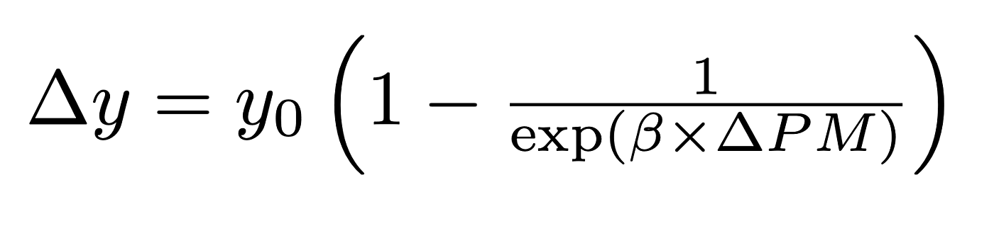
where Δy is the change in mortality, y0 is the baseline mortality rate, β is the PM2.5 coefficient, and ΔPM is the estimated change in PM2.5 design values.185 Baseline mortality is taken from the EPA’s Environmental Benefits Mapping and Analysis Program.186 The PM2.5 is the coefficient of PM2.5 estimated by Wu in their 2020 paper (0.006391) or by Pope in their 2019 paper (0.011333).187 Standard errors for Wu (0.000383) and Pope (0.001602) were used to calculate 2.5 and 97.5 percentile PM2.5 coefficients.
The economic valuation in BenMAP is calculated using a distribution of values of a statistical life (VSL) and combined with the statistical uncertainty of the PM2.5 to find a point estimate and 95 percent confidence interval. For the sake of simplicity, we used previous BenMAP results to calculate an average VSL for the 3 percent valuation point estimates and for the 2.5 and 97.5 percentile estimates. For Wu’s health impact, the VSLs for the point estimate, 2.5 percentile, and 97.5 percentile are $10,246,605, $1,046,057, and $23,998,619, respectively. For Pope’s health impact, the VSLs are $10,246,576, $1,260,962, and $21,525,586.
To simplify the results, we fold the benefits and costs of neighboring counties into their adjacent core counties. Where a neighboring county was adjacent to more than one core county we apportioned the benefits and costs to each core county. In cases where there were neighboring counties, our results therefore represent area costs and benefits. Core counties that include the effects in one or more neighboring county are denoted with an asterisk in Tables A1 and A2.
Per capita costs are calculated using estimates of resident population by county as of July 1, 2023, from the Census Bureau.188 The area population used includes the population of both core and neighborhood counties, and it is calculated the same way as the costs in each area.
Because of our simplifications, our results do not exactly match those of the EPA. However, by following its methodology relatively closely we are confident that our results reflect the overall disposition of costs and benefits on the county level. Because our estimates of avoided mortality are higher than the EPA’s, for some counties our analysis may overestimate the benefits relative to the RIA.
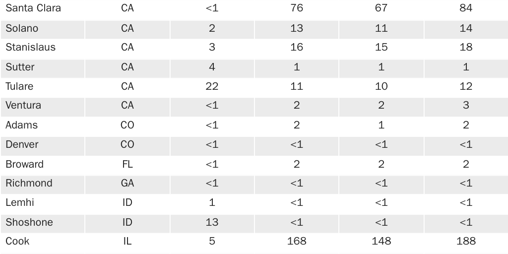
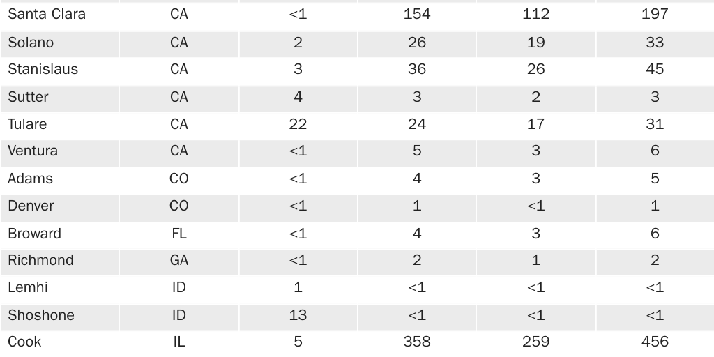
Citation
Kemp, David, and Peter Van Doren. “Rethinking Air Quality Regulation: Integrating Uncertainty, Costs, and Localized Solutions in Fine Particulate Matter Standards.” White Paper, Cato Institute, Washington, DC, July 15, 2025.

About the Authors


Notes
1. Department of Energy, “Energy Conservation Program: Energy Conservation Standards for Refrigerators, Refrigerator-Freezers, and Freezers,” Federal Register 89, no. 11, 10 CFR Part 430, RIN 1904–AF56, January 21, 2025; Department of Energy, “Energy Conservation Program: Energy Conservation Standards for Residential Clothes Washers,” Federal Register 89, no. 52, 10 CFR Part 430, RIN 1904–AF58, October 21, 2024; Environmental Protection Agency, Multi-Pollutant Emissions Standards for Model Years 2027 and Later Light-Duty and Medium-Duty Vehicles: Regulatory Impact Analysis, EPA-420-R-24–004, March 2024.
2. Office of Management and Budget, 2017 Report to Congress on the Benefits and Costs of Federal Regulations and Agency Compliance with the Unfunded Mandates Reform Act, 2017, pp. 11–12.
3. Environmental Protection Agency, “Particulate Matter (PM) Basics.”
4. Office of Management and Budget, 2017 Report to Congress on the Benefits and Costs of Federal Regulations and Agency Compliance with the Unfunded Mandates Reform Act, 2017, p. 12.
5. John Bachmann, “Will the Circle Be Unbroken: A History of the U.S. National Ambient Air Quality Standards,” Journal of the Air and Waste Management Association 57, no. 6 (June 2007): 652–97.
6. Mark Byrnes, “What Pittsburgh Looked Like When It Decided It Had a Pollution Problem,” Bloomberg, June 5, 2012.
7. John Bachmann, “Will the Circle Be Unbroken: A History of the US National Ambient Air Quality Standards,” Journal of the Air and Waste Management Association 57 (2007): 658.
8. Arthur C. Stern, “History of Air Pollution Legislation in the United States,” Journal of the Air Pollution Control Association 32, no. 1 (1982): 44.
9. John Bachmann, “Will the Circle Be Unbroken: A History of the US National Ambient Air Quality Standards,” Journal of the Air and Waste Management Association 57 (2007): pp. 652–97; and Charles O. Jones, Clean Air: The Policies and Politics of Pollution Control (University of Pittsburgh Press, 1975).
10. Jess McNally, “July 26, 1943: L.A. Gets First Big Smog,” Wired, July 26, 2010.
11. Elizabeth T. Jacobs et al., “The Donora Smog Revisited: 70 Years After the Event That Inspired the Clean Air Act,” American Journal of Public Health 108, Supplement 2 (April 2018): S85–S88.
12. W. P. D. Logan, “Mortality in the London Fog Incident, 1952,” The Lancet 261, no. 6755 (February 14, 1953): 336–38.
13. The act is described in Charles O. Jones, Clean Air: The Policies and Politics of Pollution Control (University of Pittsburgh Press, 1975), pp. 31–32.
14. John Bachmann, “Will the Circle Be Unbroken: A History of the US National Ambient Air Quality Standards,” Journal of the Air and Waste Management Association 57 (2007): 662; and Charles O. Jones, Clean Air: The Policies and Politics of Pollution Control (University of Pittsburgh Press, 1975), p. 36.
15. Arthur C. Stern, “History of Air Pollution Legislation in the United States,” Journal of the Air Pollution Control Association 32, no. 1 (1982): 51–52.
16. John Bachmann, “Will the Circle Be Unbroken: A History of the US National Ambient Air Quality Standards,” Journal of the Air and Waste Management Association 57 (2007): 662.
17. Noel de Nevers, “Air Pollution Control Philosophies,” Journal of the Air Pollution Control Association 27, no. 3 (1977): 197–218.
18. The full philosophy and the pros and cons of the different pollution control strategies are summarized by Noel de Nevers, “Air Pollution Control Philosophies,” Journal of the Air Pollution Control Association 27, no. 3 (1977): 197–218.
19. Charles O. Jones, Clean Air: The Policies and Politics of Pollution Control (University of Pittsburgh Press, 1975), pp. 78.
20. John Bachmann, “Will the Circle Be Unbroken: A History of the US National Ambient Air Quality Standards,” Journal of the Air and Waste Management Association 57 (2007): 664.
21. “The Air Quality Act of 1967,” Journal of the Air Pollution Control Association 18, no. 2 (1968), 62–71.
22. John Bachmann, “Will the Circle Be Unbroken: A History of the US National Ambient Air Quality Standards,” Journal of the Air and Waste Management Association 57 (2007): 666; and Richard L. Revesz and Jack Lienke, Struggling for Air: Power Plants and the ‘War on Coal’ (Oxford University Press, 2016), p. 50.
23. Richard L. Revesz and Jack Lienke, Struggling for Air: Power Plants and the ‘War on Coal’ (Oxford University Press, 2016), p. 32.
24. Richard Nixon, “Annual Message to the Congress on the State of the Union,” American Presidency Project, January 22, 1970.
25. Air Quality Criteria and Control Techniques, 42 U.S.C. § 7408 (2013).
26. National Primary and Secondary Ambient Air Quality Standards, 42 U.S.C. § 7409 (2013).
27. Douglas Clement, “Cost v. Benefit: Clearing the Air?,” Federal Reserve Bank of Minneapolis, December 1, 2001.
28. Whitman v. American Trucking Associations, Inc., 531 US 457 (2001), p. 465.
29. The EPA has, unsurprisingly, determined that the CAA has been successful in lowering air pollution and reducing mortality. Other commentators have argued that air pollution levels in the United States were already declining before the CAA amendments of 1970 and that alternative policies may have been more successful or cost-effective. See Environmental Protection Agency, The Benefits and Costs of the Clean Air Act 1990 to 2020 (EPA, 2011); Environmental Protection Agency, The Benefits and Costs of the Clean Air Act from 1990 to 2020: Final Report—Revised (EPA, 2011); and Joel M. Schwartz and Steven F. Hayward, Air Quality in America: A Dose of Reality on Air Pollution Levels, Trends, and Health Risks (AEI Press, 2007).
30. Environmental Protection Agency, National Air Quality Levels and Trends in Total Suspended Particulates and Sulfur Dioxide Determined by Data in the National Air Surveillance Network (EPA, 1973), pp. 28–35.
31. Environmental Protection Agency, National Air Quality and Emissions Trends Report, 1986 (EPA, 1986), pp. 4–7–4–8.
32. Environmental Protection Agency, “Air Quality Trends.”
33. Michelle L. Bell and Devra Lee Davis, “Reassessment of the Lethal London Fog of 1952: Novel Indicators of Acute and Chronic Consequences of Acute Exposure to Air Pollution,” Environmental Health Perspectives 109, Supplement 3 (2001): 389–94.
34. Short-term clinical studies on the effects of air pollution, such as those exposing subjects to ozone, have been conducted, but controlling and monitoring subjects’ exposure in the long-term is logistically unfeasible. See mention of short-term studies in Peter Van Doren, “The Fight over Particulate Matter,” Cato at Liberty (blog), April 22, 2019; and Thomas O. McGarity, “Science and Policy in Setting National Ambient Air Quality Standards: Resolving the Ozone Enigma,” Texas Law Review 93 (2015): 1783–809.
35. Environmental Protection Agency Office of Research and Development, National Center for Environmental Assessment, “Preamble to the Integrated Science Assessments,” EPA/600/R‑15/067, November 2015; and Environmental Protection Agency, Office of Research and Development, Center for Public Health and Environmental Assessment, “Supplement to the 2019 Integrated Science Assessment for Particulate Matter,” EPA/600/R‑22/028, May 2022.
36. Louis Anthony Cox Jr., Quantitative Risk Analysis of Air Pollution Health Effects (Springer, 2021); and Louis Anthony Cox Jr. and Douglas A. Popken, “Should Air Pollution Health Effects Assumptions Be Tested? Fine Particulate Matter and COVID-19 Mortality as an Example,” Global Epidemiology 2 (2020).
37. Douglas W. Dockery et al., “An Association between Air Pollution and Mortality in Six U.S. Cities,” New England Journal of Medicine 329, no. 24 (1993): 1753–59.
38. C. Arden Pope III et al., “Particulate Air Pollution as a Predictor of Mortality in a Prospective Study of US Adults,” American Journal of Respiratory and Critical Care Medicine 151, no. 3 (1994): 669–74.
39. John F. Gamble, “PM2.5 and Mortality in Long-Term Prospective Cohort Studies: Cause-Effect or Statistical Associations?,” Environmental Health Perspectives 106, no. 9 (September 1998): 535–49; and Suresh H. Moolgavkar and E. Georg Luebeck, “A Critical Review of the Evidence on Particulate Air Pollution and Mortality,” Epidemiology 7, no. 4 (July 1996): 212–13.
40. Daniel Krewski et al., “Reanalysis of the Harvard Six Cities Study and the American Cancer Society Study of Particulate Air Pollution and Mortality: Special Report,” Health Effects Institute, 2000.
41. Daniel Krewski et al., “Reanalysis of the Harvard Six Cities Study and the American Cancer Society Study of Particulate Air Pollution and Mortality: Special Report,” Health Effects Institute, 2000, table 5, p. 140.
42. Daniel Krewski et al., “Reanalysis of the Harvard Six Cities Study and the American Cancer Society Study of Particulate Air Pollution and Mortality: Special Report,” Health Effects Institute, 2000, table 21, p. 163.
43. Daniel Krewski et al., “Reanalysis of the Harvard Six Cities Study and the American Cancer Society Study of Particulate Air Pollution and Mortality: Special Report,” Health Effects Institute, 2000, table 4, p. 139, and table 21, p. 163.
44. Daniel Krewski et al., “Reanalysis of the Harvard Six Cities Study and the American Cancer Society Study of Particulate Air Pollution and Mortality: Special Report,” Health Effects Institute, 2000, p. 145.
45. Daniel Krewski et al., “Reanalysis of the Harvard Six Cities Study and the American Cancer Society Study of Particulate Air Pollution and Mortality: Special Report,” Health Effects Institute, 2000, p. 145.
46. See the discussion in Kerry Krutilla et al., “Uncertainty in the Cost-Effectiveness of Federal Air Quality Regulations,” Journal of Benefit-Cost Analysis 6, no. 1 (2015): 66–111.
47. X. Wu et al., “Evaluating the Impact of Long-Term Exposure to Fine Particulate Matter on Mortality Among the Elderly,” Science Advances 6, no. 29 (July 2020): 2–3.
48. X. Wu et al., “Evaluating the Impact of Long-Term Exposure to Fine Particulate Matter on Mortality Among the Elderly,” Science Advances 6, no. 29 (July 2020).
49. See Jonathan Wakefield, “Ecologic Studies Revisited,” Annual Review of Public Health 29, no. 1 (2008): 75–90.
50. Corey S. Sparks and Lloyd B. Potter, “Effects of Measurement Error in the American Community Survey on Statistical Analysis: An Example using County and Census Tract Mortality Rates,” 2019.
51. The ACS data are technically released by ZIP Code Tabulation Area (ZCTA). As the Census explains, “ZIP Codes and [ZCTAs] are not the same concepts. ZIP Codes are linear, as they are a collection of postal delivery routes, while ZCTAs are approximate area representations of U.S. Postal Service (USPS) 5‑digit ZIP Code service areas.” Census Bureau, American Community Survey, Technical Documentation, “2011 Geography Changes,” 2011. Wu converts ZCTA data from the ACS to zip code data in order to merge the ACS data with the rest of their data. For the sake of simplicity, we refer to the ACS data as zip code data.
52. David Raglin, “Period Estimates in the American Community Survey,” Census Bureau, March 10, 2022.
53. The issue with overlapping ACS estimates is more extensively discussed in Constance F. Citro and Graham Kalton, eds., Using the American Community Survey: Benefits and Challenges (National Academies Press, 2007); and Michael Beaghen et al., “Interpretation and Use of American Community Survey Multiyear Estimates,” Census Bureau Research Report Series Statistics no. 2012-03, April 18, 2012. The underestimation of variance is also specifically described by the Transportation Research Board, “A Guidebook for Using American Community Survey Data for Transportation Planning,” National Cooperative Highway Research Program Report no. 588, 2007, p. 104. Use of overlapping ACS five-year estimates also creates the issue of autocorrelation, but this is likely addressed by Wu’s use of bootstrapped standard errors.
54. This problem is described in Joseph L. Schafer and John W. Graham, “Missing Data: Our View of the State of the Art,” Psychological Methods 7, no. 2 (June 2002): 147–77; and Roderick J. A. Little and Donald B. Rubin, Statistical Analysis with Missing Data (Wiley & Sons, 2002).
55. See Roderick J. A. Little and Donald B. Rubin, Statistical Analysis with Missing Data (Wiley & Sons, 2002).
56. Authors’ calculation based on BRFSS data from Wu. Data are pared down to match the zip codes used in final analysis by Wu as closely as possible. However, Wu removes further zip codes based on individual-level Medicare data. Without those data we cannot be sure exactly which zip codes are used in final analysis. We base this calculation on 35,163 zip codes, while Wu includes 31,337 zip codes in their analysis.
57. The residual bias of a coarse smoking variable in a Cox proportional hazards model is described in Suresh H. Moolgavkar et al., “An Assessment of the Cox Proportional Hazards Regression Model for Epidemiologic Studies,” Risk Analysis 38, no. 4 (April 2018): 777–94. See also a more general discussion of “surrogate confounders” in Miguel A. Hernán and James M. Robins, Causal Inference: What If (Chapman and Hill/CRC, 2020), p. 94.
58. See the discussion of generalized propensity scores in Miguel A. Hernán and James M. Robins, Causal Inference: What If (Chapman and Hill/CRC, 2020), pp. 195–96.
59. Some of these are discussed in Environmental Protection Agency, “Integrated Science Assessment for Particulate Matter,” EPA/600/R‑19/188, December 2019.
60. Sonja Greven et al., “An Approach to the Estimation of Chronic Air Pollution Effects Using Spatio-Temporal Information,” Journal of the American Statistical Association 106, no. 494 (2011): 396–406.
61. Wonjun Chang et al., “A Simulation-Based Assessment of Alternative Explanations for Apparent Confounding in ‘PM Decomposition’ Studies,” Environmental Modeling & Assessment 27 (2022): 665–92.
62. We calculate county level PM2.5 as the mean of PM2.5 level of all zip codes within a county. We also weighted zip code PM2.5 levels by population density but found little difference in migration flow estimates. Migration data are from Census Bureau, American Communities Survey 2011–2015 ACS, “County-to-County Migration Flows by Age.” We use PM2.5 levels for 2015 from Wu.
63. Shilu Tong, “Migration Bias in Ecologic Studies,” European Journal of Epidemiology 16, no. 4 (April 2000): 365–69.
64. X. Wu et al., “Evaluating the Impact of Long-Term Exposure to Fine Particulate Matter on Mortality Among the Elderly,” Science Advances 6, no. 29 (July 2020): 7.
65. Limitations of the e‑value are also discussed in John P. A. Ioannidis et al., “Limitations and Misinterpretations of E‑Values for Sensitivity Analyses of Observational Studies,” Annals of Internal Medicine 170, no. 2 (January 2019): 108–11; and see the response in Tyler J. VanderWeele et al., “Correcting Misinterpretations of the E‑Value,” Annals of Internal Medicine 170, no. 2 (January 2019): 131–32.
66. Tyler J. VanderWeele and Peng Ding, “Sensitivity Analysis in Observational Research: Introducing the E‑Value,” Annals of Internal Medicine 167, no. 4 (2017): 268–74.
67. Calculated using  , where RRUD is the relative risk of mortality on the unmeasured confounder, RREU is the relative risk of the unmeasured confounder on exposure (assumed in this example to be 2.00), and RR is the observed relative risk of the outcome based on exposure (assumed to be 1.062 as found in Wu), based on Peng Ding and Tyler J. VanderWeele, “Sensitivity Analysis Without Assumptions,” Epidemiology 27, no. 3 (May 2016): 368–77.
68. Authors’ calculations based on PM2.5 exposure data by zip code from X. Wu et al., “Evaluating the Impact of Long-Term Exposure to Fine Particulate Matter on Mortality Among the Elderly,” Science Advances 6, no. 29 (July 2020).
69. Authors’ calculations using Poisson findings from X. Wu et al., “Evaluating the Impact of Long-Term Exposure to Fine Particulate Matter on Mortality Among the Elderly,” Science Advances 6, no. 29 (July 2020); and using e‑value calculator described by Maya B. Mathur et al., “Website and R Package for Computing E‑values,” Epidemiology 29, no. 5 (September 2018): e45–e47.
70. Stacey E. Alexeeff et al., “Association of Long-Term Exposure to Particulate Air Pollution with Cardiovascular Events in California,” JAMA Network Open 6, no. 2 (February 2023).
71. Authors’ calculations using PM2.5 exposure data by zip code from X. Wu et al., “Evaluating the Impact of Long-Term Exposure to Fine Particulate Matter on Mortality Among the Elderly,” Science Advances 6, no. 29 (July 2020); and Census Bureau 2016 American Communities Survey five-year estimates for population.
72. Tatyana Deryugina et al., “The Mortality and Medical Costs of Air Pollution: Evidence from Changes in Wind Direction,” American Economic Review 109, no. 12 (2019): 4178–219.
73. Wu’s estimate of a relative risk of 1.066 for a 10 μg/m3 change in PM2.5 is converted to a 1 μg/m3 by:  .
.
74. Tatyana Deryugina et al., “The Mortality and Medical Costs of Air Pollution: Evidence from Changes in Wind Direction,” American Economic Review 109, no. 12 (2019): 4211.
75. Tatyana Deryugina and Julian Reif, “The Long-Run Effect of Air Pollution on Survival,” NBER Working Paper no. 31858, November 2023.
76. See Tatyana Deryugina and Julian Reif, “The Long-Run Effect of Air Pollution on Survival,” NBER Working Paper no. 31858, November 2023, p. 35.
77. Tatyana Deryugina and Julian Reif, “The Long-Run Effect of Air Pollution on Survival,” NBER Working Paper no. 31858, November 2023, p. 16.
78. Michael L. Anderson, “As the Wind Blows: The Effects of Long-Term Exposure to Air Pollution on Mortality,” Journal of the European Economic Association 18, no. 4 (October 2019): 1886–927.
79. Alan I. Barreca et al., “Long-Run Pollution Exposure and Mortality: Evidence from the Acid Rain Program,” Journal of Public Economics 200 (August 2021).
80. Yuyu Chen et al., “Evidence on the Impact of Sustained Exposure to Air Pollution on Life Expectancy from China’s Huai River Policy,” PNAS 110, no. 32 (2013): 12936–41.
81. Avraham Ebenstein et al., “New Evidence on the Impact of Sustained Exposure to Air Pollution on Life Expectancy from China’s Huai River Policy,” PNAS 114, no. 39 (September 2017): 10384–89.
82. This is mentioned in Michael L. Anderson, “As the Wind Blows: The Effects of Long-Term Exposure to Air Pollution on Mortality,” Journal of the European Economic Association 18, no. 4 (October 2019): 35.
83. PM2.5 is a portion of both categories, and the finer particles are typically considered more dangerous than coarser particles. However, extrapolation from the observed effect of TSP or PM10 would require knowledge about the composition of airborne particulates and the relative effects of particulates of varying sizes. For example, the Air Quality Life Index uses a PM2.5-to-PM10 ratio of 0.65 based on averages of observed ratios in China during Chen’s study period. The index then uses the following conversion to translate the estimated PM10 effects (a 0.64 year reduction in life expectancy associated with a 10 μg/m3 increase in PM10):
However, this conversion ignores any effects of the coarser particulates that make up PM10 (i.e., PM2.5–10). If the assumption that all of the observed health effects of PM10 stem from the PM2.5 portion, then this conversion is correct. But, if PM2.5–10 is responsible for any of the estimated effects, this conversion overestimates the effects of PM2.5. See Air Quality Life Index, “Methodology,” Energy Policy Institute at the University of Chicago.
84. Alberto Salvo et al., “Fine-Particulate Air Pollution and Behaviorally Inclusive Mortality Impacts of China’s Winter Heating Policy, 2013–2018,” Journal of Environmental Economics and Management, 124 (March 2024).
85. See Avraham Ebenstein et al., “New Evidence on the Impact of Sustained Exposure to Air Pollution on Life Expectancy from China’s Huai River Policy,” PNAS 114, no. 39 (September 2017): table 3.
86. See Alberto Salvo et al., “Fine-Particulate Air Pollution and Behaviorally Inclusive Mortality Impacts of China’s Winter Heating Policy, 2013–2018,” Journal of Environmental Economics and Management, 124 (March 2024), table A41.
87. Authors’ calculations based on PM2.5 exposure data by zip code from X. Wu et al., “Evaluating the Impact of Long-Term Exposure to Fine Particulate Matter on Mortality Among the Elderly,” Science Advances 6, no. 29 (July 2020).
88. Michael L. Anderson, “As the Wind Blows: The Effects of Long-Term Exposure to Air Pollution on Mortality,” Journal of the European Economic Association 18, no. 4 (October 2019): 36.
89. C. Arden Pope III et al., “Fine-Particulate Air Pollution and Life Expectancy in the United States,” New England Journal of Medicine 360, no. 4 (January 2009): 376–86; and Douglas W. Dockery et al., “An Association Between Air Pollution and Mortality in Six U.S. Cities,” New England Journal of Medicine 329 (December 1993): 1753–59.
90. Tatyana Deryugina and Julian Reif, “The Long-Run Effect of Air Pollution on Survival,” NBER Working Paper no. 31858, November 2023, p. 36.
91. The decisionmaking process and rationales for the 1997, 2006, and 2013 PM2.5 National Ambient Air Quality Standards processes are described in detail in Anne E. Smith, “Setting Air Quality Standards for PM2.5: A Role for Subjective Uncertainty in NAAQS Quantitative Risk Assessments,” Risk Analysis 38, no. 11 (2018): 2318–39.
92. Juliet Eilperin and Brady Dennis, “Trump Administration Rejects Tougher Standards on Soot, a Deadly Air Pollutant,” Washington Post, December 7, 2020.
93. Lisa Friedman, “Biden Administration Toughens Limits on Deadly Air Pollution,” New York Times, February 7, 2024.
94. Authors’ calculations from Environmental Protection Agency, “Final Regulatory Impact Analysis for the Reconsideration of the National Ambient Air Quality Standards for Particulate Matter,” EPA-452/R‑24–006, January 2024, pp. 305–06.
95. C. Arden Pope III et al., “Mortality Risk and Fine Particulate Air Pollution in a Large, Representative Cohort of US Adults,” Environmental Health Perspectives 127, no. 7 (July 2019).
96. Anne E. Smith and Will Gans, “Enhancing the Characterization of Epistemic Uncertainties in PM2.5 Risk Analyses, Risk Analysis 35, no. 3 (March 2015): 361–78.
97. Environmental Protection Agency, Office of Research and Development, Center for Public Health and Environmental Assessment, “Supplement to the 2019 Integrated Science Assessment for Particulate Matter,” EPA/600/R‑22/028, May 2022, pp. 2–30–2–31.
98. See, for example, M. Brauer et al., “Exposure Misclassification and Threshold Concentrations in Time Series Analyses of Air Pollution Health Effects,” Risk Analysis 22, no. 6 (December 2002): 1183–93; and Lorenz R. Rhomberg et al., “Measurement Error in Environmental Epidemiology and the Shape of Exposure-Response Curves,” Critical Reviews in Toxicology 41, no. 8 (September 2011): 651–71.
99. Garrett Glasgow et al., “A Simulation-Based Assessment of the Ability to Detect Thresholds in Chronic Risk Concentration-Response Functions in the Presence of Exposure Measurement Error,” PLoS One 17, no. 3 (March 2022).
100. Richard T. Burnett et al., “An Integrated Risk Function for Estimating the Global Burden of Disease Attributable to Ambient Fine Particulate Matter Exposure,” Environmental Health Perspectives 122, no. 4 (April 2014): 397–403; and Bart Ostro, Outdoor Air Pollution: Assessing the Environmental Burden of Disease at National and Local Levels (World Health Organization, 2004), pp. 19–20.
101. New York City Department of Health and Mental Hygiene, “The New York City Community Air Survey: Neighborhood Air Quality 2008–2016,” 2018, table A3‑1: “Community District, Annual Average PM2.5 and Per-Year Decline in Levels.”
102. Sarath Guttikunda and Nishadh Ka, “Evolution of India’s PM2.5 Pollution Between 1998 and 2020 Using Global Reanalysis Fields Coupled with Satellite Observations and Fuel Consumption Patterns,” Environmental Science: Atmospheres 2, no. 6 (November 2022), table 3: “District (City) Average Annual PM2.5 Concentrations in μg m−3.”
103. Authors calculations based on the relative risks (RR) used by the Environmental Protection Agency in Regulatory Impact Analysis for 2024 National Ambient Air Quality Standards. The RR for Wu is 1.066 and for Pope is 1.12 for a 10 μg/m3 increase in exposure. Thus, the implied RR of a 100 μg/m3 increase in exposure is  . In terms of a 100 μg/m3 change, the relative risk estimate based on Wu 1.89 and on Pope is 3.11. Environmental Protection Agency, “Final Regulatory Impact Analysis for the Reconsideration of the National Ambient Air Quality Standards for Particulate Matter,” EPA-452/R‑24–006, January 2024, pp. 288–90.
104. The non-age-adjusted rate for New York City is taken from New York City Department of Health and Mental Hygiene, “Summary of Vital Statistics 2015,” August 2017; and the rate for Delhi is from “Annual Report on Registration of Births & Deaths in Delhi 2015,” Government of NCT of Delhi, Directorate of Economics and Statistics, July 2016.
105. This is described in C. Arden Pope III et al., “Lung Cancer and Cardiovascular Disease Mortality Associated with Ambient Air Pollution and Cigarette Smoke: Shape of the Exposure–Response Relationships,” Environmental Health Perspectives 119, no. 11 (November 2011): 1616–21.
106. Joshua S. Apte et al., “Addressing Global Mortality from Ambient PM2.5,” Environmental Science and Technology 49, no. 13 (June 2015): 8057–66.
107. X. Wu et al., “Evaluating the Impact of Long-Term Exposure to Fine Particulate Matter on Mortality Among the Elderly,” Science Advances 6, no. 29 (July 2020). And see the expanded Health Effects Institute report, Francesca Dominici et al., “Assessing Adverse Health Effects of Long-Term Exposure to Low Levels of Ambient Air Pollution: Implementation of Causal Inference Methods,” Health Effects Institute, Research Report 211, 2022.
108. Michael Brauer et al., “Mortality–Air Pollution Associations in Low-Exposure Environments (MAPLE): Phase 2,” Health Effects Institute, Research Report 212, 2022; and Bert Brunekreef et al., “Mortality and Morbidity Effects of Long-Term Exposure to Low-Level PM2.5, BC, NO2, and O3: An Analysis of European Cohorts in the ELAPSE Project,” Health Effects Institute, Research Report 208, 2021.
109. Suresh H. Moolgavkar, “Fine Particulate Matter Pollution and Mortality,” Risk Analysis 36, no. 9 (2016): 1766–69.
110. Garrett Glasgow et al., “Model Misspecification, Measurement Error, and Apparent Supralinearity in the Concentration-response Relationship Between PM2.5 and Mortality,” PLoS One 19, no. 5 (May 2024): e0303640.
111. The chemical reactions and the interactions between different precursor gases and particulates of varying sizes are described in detail in Christian Seigneur, “Atmospheric Particles,” chap. 9 in Air Pollution: Concepts, Theory, and Applications (Cambridge University Press, 2019): 190–238.
112. Environmental Protection Agency, “Integrated Science Assessment for Particulate Matter,” EPA/600/R‑19/188, December 2019, pp. 2–13.
113. George D. Thurston et al., “A Source Apportionment of U.S. Fine Particulate Matter Air Pollution,” Atmospheric Environment 45, no. 24 (2011): 3924–36.
114. Environmental Protection Agency, “Integrated Science Assessment for Particulate Matter,” EPA/600/R‑19/188, December 2019, pp. 2–59–2–62.
115. Bin Cheng et al., “Spatiotemporal Trends in PM2.5 Chemical Composition in the Conterminous US During 2006–2020,” Atmospheric Environment 316 (January 2024).
116. R. E. Wyzga and A. C. Rohr “Long-Term Particulate Matter Exposure: Attributing Health Effects to Individual PM Components,” Journal of the Air and Waste Management Association 65, no. 5 (May 2015): 523–43.
117. Environmental Protection Agency, “Integrated Science Assessment for Particulate Matter,” EPA/600/R‑19/188, December 2019, pp. 11–93.
118. Minhan Park et al., “Differential Toxicities of Fine Particulate Matters from Various Sources,” Scientific Reports 8, no. 1 (November 2018).
119. Alistair Thorpe and Roy M. Harrison, “Sources and Properties of Non-Exhaust Particulate Matter from Road Traffic: A Review,” Science of the Total Environment 400, nos. 1–3 (2008): 270–82.
120. David Scott Williams et al., “Particulate Matter Emission by a Vehicle Running on Unpaved Road,” Atmospheric Environment 42, no. 16 (May 2008): 3899–905.
121. Magdalena Penkała et al., “Particulate Matter from the Road Surface Abrasion as a Problem of Non-Exhaust Emission Control,” Environments 5, no. 1 (January 2018).
122. See, for example, Yifan Wang et al., “Long-Term Exposure to PM2.5 Major Components and Mortality in the Southeastern United States,” Environment International 158 (January 2022); Tingfan Jin et al., “Associations Between Long-Term Exposures to Airborne PM2.5 Components and Mortality in Massachusetts: Mixture Analysis Exploration,” Environmental Health 21 (October 2022); and Priyanka deSouza et al., “Associations Between Ambient PM2.5—Components and Age-Specific Mortality Risk in the United States,” Environmental Advances 9 (October 2022).
123. Neil J. Hime et al., “A Comparison of the Health Effects of Ambient Particulate Matter Air Pollution from Five Emission Sources,” International Journal of Environmental Research and Public Health 15, no. 6 (June 2018).
124. George D. Thurston et al., “Ischemic Heart Disease Mortality and Long-Term Exposure to Source-Related Components of U.S. Fine Particle Air Pollution,” Environmental Health Perspectives 124, no. 6 (June 2016): 785–94.
125. Ruimang Liang et al., “Associations of Long-Term Exposure to Fine Particulate Matter and Its Constituents with Cardiovascular Mortality: A Prospective Cohort Study in China,” Environment International 162 (April 2022).
126. See description in Kate Adams et al., “Particulate Matter Components, Sources, and Health: Systematic Approaches to Testing Effects,” Journal of the Air and Waste Management Association 65, no. 5 (May 2015): 544–58.
127. See list of regulations included in Environmental Protection Agency’s baseline projections: Environmental Protection Agency, “Final Regulatory Impact Analysis for the Reconsideration of the National Ambient Air Quality Standards for Particulate Matter,” EPA-452/R‑24–006, January 2024, pp. 39–40.
128. Authors’ calculations from Environmental Protection Agency, “Final Regulatory Impact Analysis for the Reconsideration of the National Ambient Air Quality Standards for Particulate Matter,” EPA-452/R‑24–006, January 2024, pp. 187 and 258.
129. Anne E. Smith and Will Gans, “Enhancing the Characterization of Epistemic Uncertainties in PM2.5 Risk Analyses,” Risk Analysis 35, no. 3 (March 2015): 361–78.
130. Marshall Burke et al., “The Changing Risk and Burden of Wildfire in the United States,” PNAS 118, no. 2 (January 2021); and J. L. Hand et al., “Spatial and Seasonal Variability in Fine Mineral Dust and Coarse Aerosol Mass at Remote Sites Across the United States,” Journal of Geophysical Research: Atmospheres 122, no. 5 (March 2017): 3080–97.
131. Qiang Zhang et al., “Transboundary Health Impacts of Transported Global Air Pollution and International Trade,” Nature 543 (March 2017): 705–09.
132. Government Accountability Office, “Information on Tall Smokestacks and Their Contribution to Interstate Transport of Air Pollution,” GAO-11–473, May 11, 2011.
133. Ying Zhou and Jonathan Levy, “Factors Influencing the Spatial Extent of Mobile Source Air Pollution Impacts: A Meta-Analysis,” BMC Public Health 7, no. 89 (May 2007).
134. Background particulate matter levels are summarized in Environmental Protection Agency, “Integrated Science Assessment for Particulate Matter,” EPA/600/R‑19/188, December 2019, pp. 2–90–2–93.
135. See Marco Pandolfi et al., “Long-Range and Local Air Pollution: What Can We Learn from Chemical Speciation of Particulate Matter at Paired Sites?,” Atmospheric Chemistry and Physics 20, no. 1 (January 2020): 409–29; and Jerome E. McGinnis et al., “Understanding the Sources and Composition of the Incremental Excess of Fine Particles Across Multiple Sampling Locations in One Air Shed,” Journal of Environmental Sciences 26, no. 4 (April 2014): 818–26.
136. Eugene Kim et al., “Sources of Fine Particles in a Rural Midwestern U.S. Area,” Environmental Science and Technology 39, no. 13 (July 2005): 4953–60.
137. Pablo Garcia Rivera et al., “Source-Resolved Variability of Fine Particulate Matter and Human Exposure in an Urban Area,” Atmospheric Chemistry and Physics 22, no. 3 (February 2022). See also A. Polidori et al., “Source Proximity and Residential Outdoor Concentrations of PM2.5, OC, EC, and PAHs,” Journal of Exposure Science & Environmental Epidemiology 20, no. 5 (July 2010): 457–68.
138. Neal Fann et al., “The Influence of Location, Source, and Emission Type in Estimates of the Human Health Benefits of Reducing a Ton of Air Pollution,” Air Quality, Atmosphere, and Health 2, no. 3 (September 2009): 169–76.
139. Sebastien Humbert et al., “Intake Fraction for Particulate Matter: Recommendations for Life Cycle Impact Assessment,” Environmental Science and Technology 45, no. 11 (June 2011): 4808–16.
140. Environmental Protection Agency, “Final Regulatory Impact Analysis for the Reconsideration of the National Ambient Air Quality Standards for Particulate Matter,” EPA-452/R‑24–006, January 2024, pp. 64–65.
141. Provat K. Saha et al., “Hyper-Local to Regional Exposure Contrast of Source-Resolved PM2.5 Components Across the Contiguous United States: Implications for Health Assessment,” Journal of Exposure Science & Environmental Epidemiology 34, no. 5 (September 2023): 836–44.
142. Environmental Protection Agency, “Final Regulatory Impact Analysis for the Reconsideration of the National Ambient Air Quality Standards for Particulate Matter,” EPA-452/R‑24–006, January 2024, p. 189.
143. R. U. Shah et al., “Socio-Economic Disparities in Exposure to Urban Restaurant Emissions Are Larger than for Traffic,” Environmental Research Letters 15, no. 11 (2020).
144. Design values are defined in “Appendix N to Part 50—Interpretation of the National Ambient Air Quality Standards for PM2.5,” 40 C.F.R. § 50 (1971).
145. The methods used are summarized in Environmental Protection Agency, “Final Regulatory Impact Analysis for the Reconsideration of the National Ambient Air Quality Standards for Particulate Matter,” EPA-452/R‑24–006, January 2024, pp. 45–46.
146. Other analyses have found that more counties will be affected, such as an analysis by the Chamber of Commerce that determined that, based on PM2.5 levels from 2021 to 2023, 569 counties would be in non-attainment with the 9 μg/m3 standard. However, the Chamber of Commerce includes the effects of wildfires, which, according to how the Environmental Protection Agency calculates design values, should be excluded. Chamber of Commerce, “EPA’s Proposed Air Quality Standards Will Cause Permitting Gridlock across Our Economy,” November 9, 2023.
147. Environmental Protection Agency, “Nonattainment Areas for Criteria Pollutants (Green Book).”
148. Richard L. Revesz, “Air Pollution and Environmental Justice,” Ecology Law Quarterly 49, no. 187 (2022): pp. 239–40.
149. Environmental Protection Agency, “Nonattainment NSR Basic Information.”
150. Randy A. Becker, “Air Pollution Abatement Costs Under the Clean Air Act: Evidence from the PACE Survey,” Journal of Environmental Economics and Management 50, no. 1 (July 2005): 144–69.
151. Randy A. Becker and J. Vernon Henderson, “Costs of Air Quality Regulation,” in Carlo Carraro and Gilbert E. Metcalf, eds., Behavioral and Distributional Effects of Environmental Policy (Chicago University Press, 2001), pp. 159–86.
152. Randy Becker and Vernon Henderson, “Effects of Air Quality Regulations on Polluting Industries,” Journal of Political Economy 108, no. 2 (April 2000): 379–421.
153. Michael Greenstone, “The Impacts of Environmental Regulations on Industrial Activity: Evidence from the 1970 and 1977 Clean Air Act Amendments and the Census of Manufactures,” Journal of Political Economy 110, no. 6 (December 2002): 1175-219.
154. Michael Greenstone, “The Impacts of Environmental Regulations on Industrial Activity: Evidence from the 1970 and 1977 Clean Air Act Amendments and the Census of Manufactures,” Journal of Political Economy 110, no. 6 (December 2002): 1212.
155. Michael Greenstone et al., “The Effects of Environmental Regulation on the Competitiveness of U.S. Manufacturing,” MIT Department of Economics Working Paper no. 12–24, September 2012.
156. W. Reed Walker, “The Transitional Costs of Sectoral Reallocation: Evidence from the Clean Air Act and the Workforce,” Quarterly Journal of Economics 128, no. 4 (November 2013): 1787–835.
157. Authors’ calculations are from Environmental Protection Agency, “PM2.5 Design Values,” Office of Air Quality Planning and Standards.
158. Authors’ calculations are based on control cost data by county used in the Regulatory Impact Analysis and shared by the Environmental Protection Agency. Environmental Protection Agency, “Final Regulatory Impact Analysis for the Reconsideration of the National Ambient Air Quality Standards for Particulate Matter,” EPA-452/R‑24–006, January 2024.
159. The 10 counties, in order of annual avoided mortality, are Los Angeles County, California; Allegheny County, Pennsylvania; Cook County, Illinois; Harris County, Texas; Maricopa County, Arizona; Delaware County, Pennsylvania; Wayne County, Michigan; Alameda County, California; Santa Clara County, California; and Cuyahoga County, Ohio. See the appendix.
160. Shoshone County, Idaho, is estimated to have negative net benefits except at the 97.5 percentile for the Pope mortality impact.
161. Peter Van Doren, “When and How We Should ‘Trust the Science,’” Cato Institute, Pandemics and Policy, September 15, 2020.
162. National Research Council, Estimating the Public Health Benefits of Proposed Air Pollution Regulations (National Academies Press, 2002), p. 126.
163. Art Fraas and Randall Lutter, “Uncertain Benefits Estimates for Reductions in Fine Particle Concentrations,” Risk Analysis 33, no. 3 (March 2012): 434–49.
164. Anne E. Smith and Will Gans, “Enhancing the Characterization of Epistemic Uncertainties in PM2.5 Risk Analyses,” Risk Analysis 35, no. 3 (March 2014): 361–78.
165. Anne E. Smith, “Setting Air Quality Standards for PM2.5: A Role for Subjective Uncertainty in NAAQS Quantitative Risk Assessments?,” Risk Analysis 38, no. 11 (August 2018): 2318–39.
166. Henry A. Roman et al., “Expert Judgment Assessment of the Mortality Impact of Changes in Ambient Fine Particulate Matter in the U.S.,” Environmental Science & Technology 42, no. 7 (February 2008): 2268–74.
167. Noel de Nevers, “Air Pollution Control Philosophies,” Journal of the Air Pollution Control Association 27, no. 3 (1977): 200.
168. Noel de Nevers, “Air Pollution Control Philosophies,” Journal of the Air Pollution Control Association 27, no. 3 (1977): 201–02.
169. Michael A. Livermore and Richard L. Revesz, “Rethinking Health-Based Environmental Standards,” New York University Law Review 89, no. 4 (2014): 1187–88.
170. Cary Coglianese and Gary E. Marchant, “Shifting Sands: The Limits of Science in Setting Risk Standards,” University of Pennsylvania Law Review 152, no. 4 (April 2004): 1255-360.
171. See Cary Coglianese and Gary E. Marchant, “Shifting Sands: The Limits of Science in Setting Risk Standards,” University of Pennsylvania Law Review 152, no. 4 (April 2004): 1356.
172. Brian Sergi et al., “Regional and County Flows of Particulate Matter Damage in the US,” Environmental Research Letters 15, no. 10 (October 2020).
173. Andrew L. Goodkind et al., “Fine-Scale Damage Estimates of Particulate Matter Air Pollution Reveal Opportunities for Location-Specific Mitigation of Emissions,” Environmental Sciences 116, no. 18 (April 2019): 8775–80.
174. John M. Morehouse and Edward Rubin, “Downwind and Out: The Strategic Dispersion of Power Plants and Their Pollution,” Center for Growth and Opportunity at Utah State University working paper, May 2021; and J. E. Monogan III et al., “Gone with the Wind: Federalism and the Strategic Location of Air Polluters,” American Journal of Political Science 61, no. 2 (April 2017): 257–70.
175. 42 U.S.C. § 7410(a)(2)(D), (2025).
176. Richard L. Revesz, “Air Pollution and Environmental Justice,” Ecology Law Quarterly 49, no. 187 (2022): 248–50.
177. Ohio v. Environmental Protection Agency, No. 23A349 (US 2024). Argued February 21, 2024; decided June 27, 2024.
178. See Joseph E. Aldy et al., “Looking Back at 50 Years of the Clean Air Act,” NBER Working Paper no. 26687, revised December 2020; and Richard Schmalensee and Robert N. Stavins, “Lessons Learned from Three Decades of Experience with Cap and Trade,” Review of Environmental Economics and Policy 11, no. 1 (Winter 2017): 59–79.
179. Richard L. Revesz, “The Race to the Bottom and Federal Environmental Regulation: A Response to Critics,” Minnesota Law Review 82, no. 2 (December 1997): 541.
180. Environmental Protection Agency, “Final Regulatory Impact Analysis for the Reconsideration of the National Ambient Air Quality Standards for Particulate Matter,” EPA-452/R‑24–006, January 2024, pp. 54–55.
181. David Schoenbrod, “Why States, Not EPA, Should Set Pollution Standards,” Regulation 19, no. 4 (1996): 21.
182. David Schoenbrod, “Why States, Not EPA, Should Set Pollution Standards,” Regulation 19, no. 4 (1996): 21.
183. Peter Van Doren, “Letting Environmentalists’ Preferences Count,” Regulation 26, no. 3 (Fall 2003): 32–35.
184. Environmental Protection Agency, “Final Regulatory Impact Analysis for the Reconsideration of the National Ambient Air Quality Standards for Particulate Matter,” EPA-452/R‑24–006, January 2024, p. 67.
185. Log-linear health impact functions are described in Environmental Protection Agency, “Environmental Benefits Mapping and Analysis Program User’s Manual Version 0.5,” April 2024, pp. C‑6–C‑8.
186. Environmental Protection Agency, “Environmental Benefits Mapping and Analysis Program—Community Edition (BenMAP-CE).”
187. Environmental Protection Agency, “Environmental Benefits Mapping and Analysis Program User’s Manual Version 0.5,” April 2024, p. E‑2.
188. Census Bureau, “County Population Totals and Components of Change: 2020–2023,” Annual Estimates of the Resident Population for Counties: April 1, 2020, to July 1, 2023 (CO-EST2023-POP).

This work is licensed under a Creative Commons Attribution-NonCommercial-ShareAlike 4.0 International License.